cfd analysis

To simulate rotating motion, like for wind turbines or pumps, in a CFD analysis can be cumbersome. It requires full temporal and spatial discretization of flow around moving objects with carefully selected time-steps to capture the movement and often an interface to separate the moving region from the stationary domain. Sometimes, when you are primarily interested in the detailed flow characteristics around the propeller, fan or pump, there is no shortcut passing rigid body motion simulations. However, in Simcenter STAR-CCM+ there are some simplified approaches available which model the effect of rotating machinery and are easy to setup, time efficient, and less  computationally expensive. In this first blog on Rotating Flow I intend to give you a brief overview of the Fan Modelling methods.

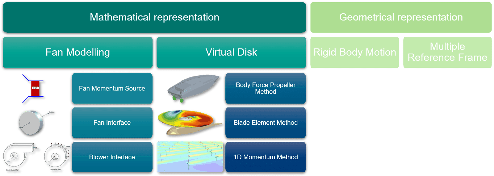
So, here we focus on the simplified approaches which model rather the effect of the rotating parts than the rotating parts themselves. We model their effect on the surrounding flow field mathematically by adding volumetric body forces to the momentum equations or by imposing a pressure jump across a plane surface. In blog Rotating Flow part II, we will cover the Virtual Disk methods.

Fan modelling

The three fan models are particular useful for simulation when the exact geometry of the fan is either not known or not important for the cfd analysis. What is needed is, however, the fan performance curve which relates the pressure rise to flow rate or velocity. Such distribution can simply be imported from a csv file into a File Table.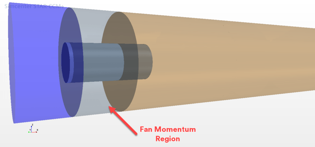

Here we have a simple test scenario with a fan just behind the stagnation inlet inside of a pipe. Fan modelling can be applied through a plane surface (Fan Interface and Blower Interface) or a volumetric region (Fan Momentum Source). The Fan Momentum Source models the fan as a volumetric region and introduce sources in the momentum equation to model pressure rise and swirl. The total source term is thereby the sum of an axial and tangential force term. The tangential component is calculated by considering the velocity vector on a single fan blade. While the blade angle is assumed to be constant in radial direction. The axial component is calculated such that a target pressure raise is achieved. While the target pressure follows the fan curve for the given mass flow rate between inlet and outlet of the fan region. Unlike the Fan Interface method, here we have to provide the fan performance as volumetric flow rate in [m^3/s] and pressure rise in [pa].

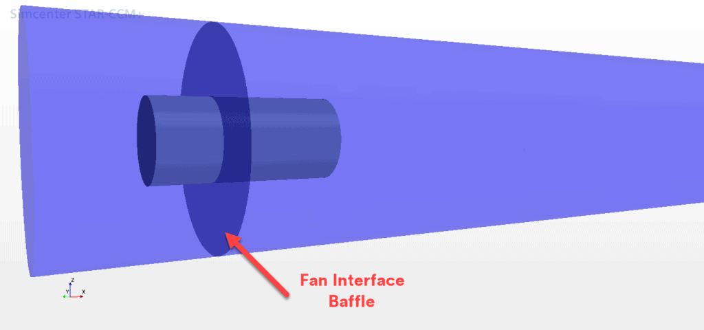
Fan Interface is a model that represents an axial fan by a zero-thickness interface and imposes a pressure jump across the interface. The pressure jump is obtained from a user-specified fan curve that plots pressure jump as a function of flow rate or flow velocity. This can be the same as for the Fan Momentum. However, for the Fan Interface you can alternatively provide a fan curve from a Polynomial.

The Fan Interface can also add swirl to the flow downstream of the fan. In CFD analysis Swirl is in this method obtained either from the fan efficiency or from user defined velocity component. The fan efficiency formulation yields a quadratic equation for the tangential velocity component. Simcenter STAR-CCM+ uses only the negative square root. Which sort of determines the final rotation direction.

The Blower Interface, the third method among the fan modelling, is a non-conformal interface that connects the inlet and the outlet of the impeller or the centrifugal fan. Unlike an axial fan, an impeller or a centrifugal fan has the inlet and the outlet located in different places and oriented in different directions. As for the Fan Interface is the fan effect modelled by a pressure jump across the interface. The pressure jump again obtained by fan curve that plots pressure jump as a function of volumetric flow rate. The inside of the fan can be omitted when discretizing.

Generally, the Fan Interface is more robust, and it is usually recommended over the fan momentum source. The method works straight forward without detailed information of the fan geometry and an easy setup for a single region. Swirl modelling is, however, rather difficult for both method and depends on user specified input. In the video below you can see that both methods yield different swirl and consequently different velocity distributions. The swirl can be represented in more detailed with the Fan Interface method thanks to User-Specified Fan Swirl that can be varying in radial direction distribution. The next step of simulation fidelity would be the Virtual Disk which offers broader range of control option for a range of application areas. This will be discussed in Rotating Flow part II. I hope this has given you a brief introduction to the possibilities of simulating rotating flow within Simcenter Star-CCM+. More information can be obtained in the documentation. And as usual, if you have any questions, do not hesitate to reach out at support@volupe.com.

Read also:
Rotating flow Part 2
Who wants innovation