Drag coefficients
On this page, we have summarized
- Shapes and corresponding drag coefficients.
- Description of how the drag coefficient depends on fluid flow properties.
- Recommended simulation setup for calculations of drag and lift coefficients in Simcenter STAR-CCM+.
Shapes and corresponding drag coefficients
See table below for drag coefficients for different shapes in both 2D and 3D. The bodies are assumed to be smooth (no surafece roughness) with flow from left to right. Data is mainly obtained from White [1] where the drag coefficients are based on experimental data, but other sources are also used [2, 3].
SHAPE
DIMENSION
Visualization of shape
Drag coefficient at Re ~10^4
CIRCLE
2D

1.17
Half circle with rounded side downstream
2D

1.7
Half circle with rounded side upstream
2D

1.2
Square
2D

2.1
Square rotated 45degrees
2D

1.6
Flat horizontal plate
2D

2.0
Triangle with the pointy end pointing downstream (equilateral, 60 degrees angels)
2D

2.0
Triangle with the pointy end pointing upstream (equilateral, 60 degrees angels)
2D

1.6
Airfoil (streamlined body)
2D

0.045
Sphere
3D

0.47
Half sphere with the rounded part downstream
3D

1.15
Half sphere with the rounded part upstream
3D

0.42
Short cylinder with flat end in the flow direction (flat plate)
3D

1.28
Long cylinder with flat end in the flow direction (length 6 times the diameter)
3D

0.95
Cube with flat end in the flow direction
3D

1.07
Cube with sharp edge in the flow direction
3D

0.81
Cone which has the pointy edge downstream
(30 degrees between the leaning surfaces)
3D

1.15
Cone with the pointy edge upstream, based on angle between the leaning surfaces.
10, 20, 30, 40, 60, 75 and 90 degrees
3D

Angle in degrees ; Drag coefficient
10 ; 0.3
20 ; 0.4
30 ; 0.55
40 ; 0.65
60 ; 0.8
75 ; 1.05
90 ; 1.15
The drag coefficient C_d is defined as
C_d = \frac{2 F_d}{\rho u^2 A}
where F_d is the drag force component in the direction of the flow velocity, ρ is the density of the fluid, u is the flow speed relative to the object and A is the reference area. Reference area is often the same as projected frontal area, but for bodies that vary in cross-sectional shape this might not be the case. For exemple, airfoils has the reference area of the nominal wing area.
The drag force can be divided into two components which are frictional drag (viscous drag) and pressure drag (drag based on shape). Some of the bodies in the table above would be described as blunt/bluff bodies, and these are the ones where pressure drag is the main component of the drag force. The shape of bluff bodies is defined as a shape where high pressure gradients in the flow field around it occurs (separation often occurs as well) – which is often leading to high drag. Friction is often a small component of drag, but when having streamlined bodies, this can still be the major contributor to drag since no separation occurs – this will be the case of low drag bodies.
One field where drag calculations are of high importance is the automotive industry, where improving aerodynamics (reducing drag) is important to reduce fuel consumption. The shape of cars have developed a lot during the years and the first car that was released to the market was shaped like a box and had therefore high pressure drag. The low speed of the first cars did not demand a streamlined shape, but nowadays the streamlined shape is used when designing cars. The drag coefficient has gone down from around 0,95 to 0,3. Drag coefficients for different car models can be found on Wikipedia where cars are listed, for example an Audi A3 has a C_d of 0,33 while a Tesla model S has a value of 0.24 [4].
Drag coefficient dependencies based on fluid properties
The shape of a body is one of the most important properties for the flow field when looking at drag, but there are several more properties that can affect the drag. Some of the properties are discussed below.
Reynolds number
Due to fluid phenomenon occurring when going from laminar to turbulent flow, it may feel intuitive that velocity of the flow will affect the drag. In the previous section when discussing the drag coefficient you could see that a term of the squared velocity will be included in the expression when calculating C_d. The relation between drag and flow velocity is more complicated though, since when varying flow properties turbulence and eddies will get different structure. The structure is dependent on Reynolds number and therefore the table above only looking at one specific Reynolds number (10^4). If we allow the Reynolds number to vary every shape will have a unique dependency when determining the drag coefficient. For example, a sphere will have a higher drag at low Reynolds numbers and lower drag at higher Reynolds numbers, as seen in the picture below [2]. Reed more about Reynolds number and other dimensionless fluid properties at the Volupe web page for dimensionless numbers.
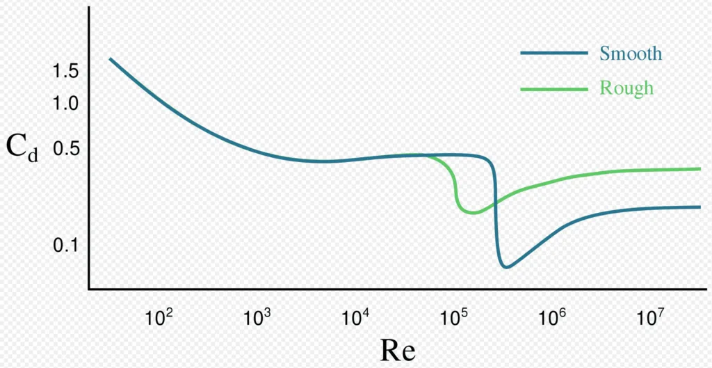
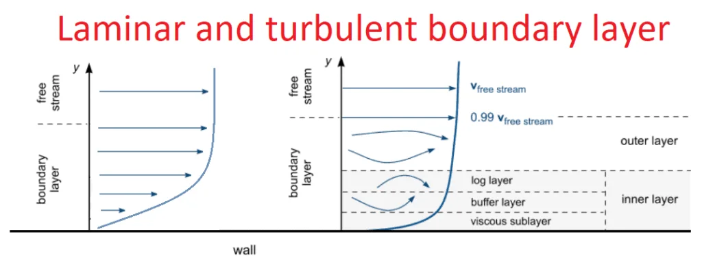
As you can see in the picture above the surface roughness will also affect the drag. The roughness of the surface will affect the boundary layer and therefore the velocity of the fluid close to the surface. In the picture below you can see the velocity in the boundary layer as a function of distance to the wall – for laminar and turbulent flow.
Golf ball example
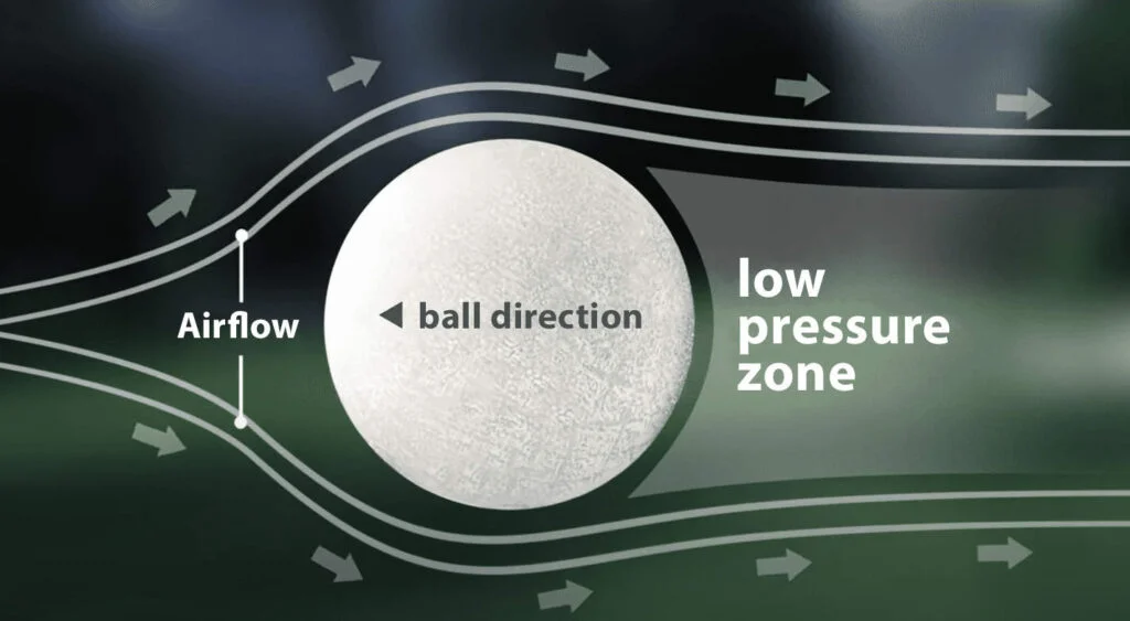
One example of the impact for surface appearance, when looking at drag, is the fluid flow around a golf ball. In the picture below you can see the flow around a smooth golf ball, where flow around the ball is moving from left to right. The low pressure region behind the ball, the wake, is large and creating a suction effect which will slow the ball down.
When adding dimples, the wake region is decreased a lot, which can be seen in the picture below. The dimples are creating a turbulent boundary layer which will reattach the separated flow to the ball surface. This means that flow will follow the ball instead of creating the wake region, which will results in much less drag – and this can help the ball reaching double the distance compared to the distance the smooth ball.
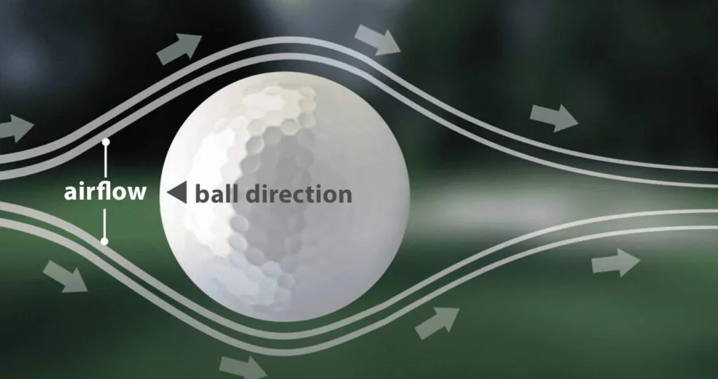
The pictures regarding the golf balls example were retrieved from [5], where further explanation of how the dimples are affecting the flow can be found. And there it is also explained that dimples also increase the lifting affect, since the flow around the wake will more easily be directed downwards (if the ball is spinning counter clockwise in the picture below) instead of having the flow around the wake aligned with the ball direction.

Recommended simulation set up for calculations of drag and lift coefficients in Simcenter STAR-CCM+
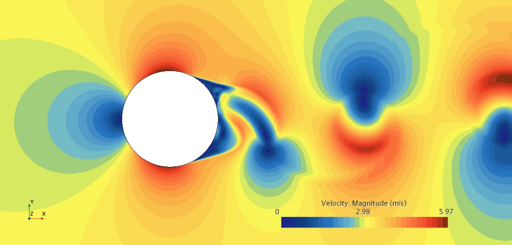
Calculating lift and drag coefficients includes complicated physics where near wall properties of the flow must be resolved to high extent. Everything in the set-up, from mesh resolution to choose of turbulence models, has to be set up with highest accuracy to capture the fluid phenomenon which give rise to lift and drag on the body. The picture below shows the phenomenon of a von Karman vortex street behind a cylinder (flow from left to right).
Computational domain
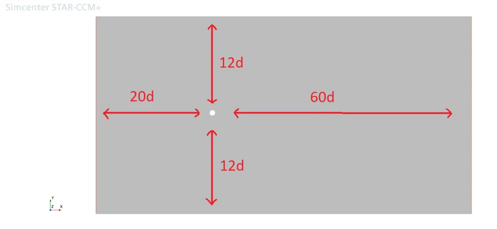
The first thing you have to decide when running drag coefficient calculations is the size of the fluid domain. The dimensions of the fluid domain can be described in terms of the characteristic length of the body of interest. In the case of running a simulation for drag of a cylinder the computational domain should have 12d between the walls around the cylinder, where d is the diameter of the cylinder. This length is for the wall not to affect the flow field. Before the cylinder (left wall in picture below) a distance of 20d should be used for the boundary condition on the inlet not to force the flow field in front of the cylinder to obtain a distribution prescribed at the inlet. Behind the 60d should be used to not to affect the flow field after the body. [6]
Mesh settings
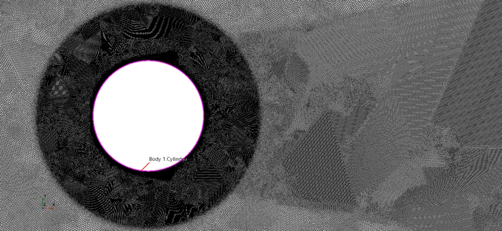
When discretizing the fluid domain you want to resolve the fluid properties to a high enough level, but just to be sufficient, in order to not spend more computational resources than needed. Meaning that finer cells will be needed where gradients in the flow field occur. Looking at the picture below, finer cells are needed closer to the cylinder, to resolve the gradients close to the wall and in the wake region.
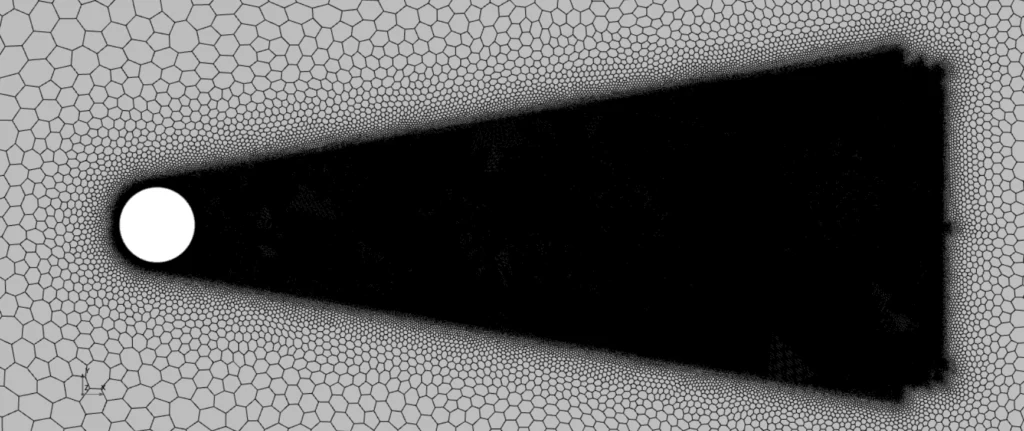
Below an example of a zoomed-out picture on a wake refinement is shown (note that picture is meant to visualize the feature of wake refinement and that the mesh resolution in front of the cylinder is note resolved enough for a drag and lift coefficient simulation). This feature requires an input in form of a surface to refine from, and then resolution, length of the resolution and angle of spread can be defined to customize the refinement.
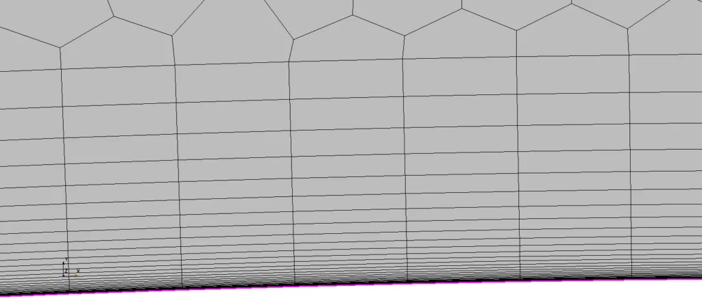
When focusing on the near wall mesh, the prism layers should provide a first cell resulting in a y+ value below 1, enough layers to cover the boundary layer, stretching factor of 1.1 to 1.2 (meaning height of prism layer cells growing with 10% to 20% outwards from the wall) and the transition to the bulk mesh should result in the last prism layer cell of equal height as the first bulk mesh size. To make sure to fulfill these criteria you can use the y+ calculator we at Volupe developed. See example on a good prism layer mesh below.
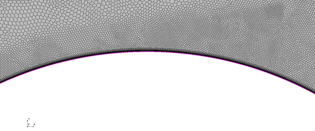
The mesh close to the cylinder then look like the picture below when zoomed out a bit.
Turbulence models
The discretization of the fluid domain gives conditions for turbulence models to resolve the physics. For such complex physics as turbulence there are many different models that you can chose between. Among the less accurate models k-omega SST is one to recommend due to its accurate predictions of the near wall treatment and efficient bulk flow predictions [1]. The most accurate result you will of course get if you use more expensive models, that resolve the turbulent eddies in more detail, for example LES. LES demands both fine mesh resolution and short time steps, and without fulfilling recommended settings an k-omega SST simulation can provide better predictions than LES. You find the guidelines for LES in the Simcenter STAR-CCM+ documentation at Simcenter STAR-CCM+ -> Simulating physics -> Turbulence -> Scale-resolving simulations -> Large eddy simulation (LES) -> LES guidelines.
Evaluating the results
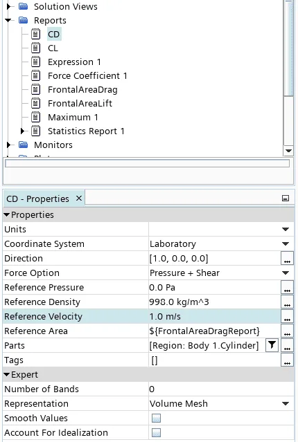
To be able to evaluate the results from your simulation you need to visualize the data you are calculating. Visualizing flow fields are powerful to get a feeling about the physical phenomenon, but one of the absolute strongest ways of evaluating the simulation is to set up reports and monitor them via plots. There is built in reports for lift and drag coefficients which you define based on:
- flow direction (specified in terms of components)
- fluid density
- relative fluid velocity (free stream velocity)
- frontal area of the body (can be determined via an area report)
See picture below for how to define one of these reports.
When you are running simulations with fluctuations in the flow field you have the possibility to filter out the disturbances in data via mean field monitors. In the later part of this Volupe blog post it is shown How to create a mean field monitor.
Reference list
[1] Fluid mechanics seventh edition, Frank M White, 2008, USA.
[2] Drag coefficient, Wikipedia, https://en.wikipedia.org/wiki/Drag_coefficient, 2021.
[3] Shape effects on drag, NASA, https://www.grc.nasa.gov/www/k-12/airplane/shaped.html, 2021.
[4] Automotive drag coefficient, Wikipedia, https://en.wikipedia.org/wiki/Automobile_drag_coefficient, 2022.
[5] Science of golf: Why golf balls have dimples, United states golf association (USGA) at Youtube, https://www.youtube.com/watch?v=fcjaxC-e8oY, 2015.
[6] Numerical Analysis of Drag Force Acting on 2D Cylinder Immersed in Accelerated Flow, Hyun A. Son and Sungsu Lee and Jooyong Lee, June 2020, Korea.
About the web page for drag coefficients
This web page about drag coefficients is developed from us at Volupe, to help you being able to use your simulation software in the best way possible.
If you have any questions about your simulation, or ideas for this web page, feel free to contact us at support@volupe.com or give me (Christoffer) a call via the contact information below. Your feedback is important for us!