y+ calculator
Find the first cell height for a target y+, then size the boundary layer and prism layer stack for Simcenter STAR-CCM+.
What is y+?
y+ (y plus) is the dimensionless distance from a wall, y+ = uτy/ν. In a CFD simulation you check it at the centre of the first cell next to the wall, because it tells you which layer of the turbulent boundary layer that cell sits in, and so how fine the wall mesh has to be.
uτ = √(τw / ρ)
Here uτ is the friction velocity, y the distance from the wall to the cell centre, ν the kinematic viscosity, τw the wall shear stress and ρ the density. Aim for a y+ of about 1 or less if you resolve the viscous sublayer with a low-y+ wall treatment, and 30 to 300 if you use wall functions. Siemens advises 30 to 150 for most wall-function cases, and higher values in some applications such as marine flows. Avoid 5 to 30, the buffer layer, where neither approach is accurate. The upper limit of 300 comes down at low Reynolds numbers, where the log layer is short. Which y+ should you aim for? gives the targets for each wall treatment.
Before a simulation you do not know τw, so the calculator estimates it from a skin-friction correlation: a turbulent flat-plate correlation for external flow, the Blasius friction law for smooth pipes. It then gives you the first cell height, twice the cell-centre distance, for the y+ you choose. After the run, check the actual y+ on the walls and adjust the prism layer if needed.
How to use the y+ calculator
1. Choose the fluid and the flow type. External flow runs over a body; internal flow runs through a pipe or duct. Air and water at 20 °C fill in density and viscosity. Choose Custom for anything else.
2. Enter the velocity, the reference length and the y+ you want at the wall. The first cell height Δy1 updates as you type. This is the value to use as the prism layer near-wall thickness. Already have a mesh? Switch “Solve for” to y+ of my mesh and enter its first cell height to see the y+ it gives.
3. Check the boundary layer thickness in step 2. Step 3 then shows how much of it your prism layer covers and how many layers would reach its edge. Siemens advises that the prism layers ideally cover the whole boundary layer, with a total thickness of about the boundary-layer height.
4. Set the stretching ratio and the number of layers in step 3, then copy the values into the prism layer default controls of your automated mesh operation. In step 4, compare the last layer with your core mesh size, so the mesh grows smoothly away from the wall. The chart in step 3 shows where each cell centre sits on the law of the wall.
Which y+ should you aim for?
The right target depends on how your turbulence model treats the wall. For large eddy simulation (LES), Siemens advises a y+ of around 1.
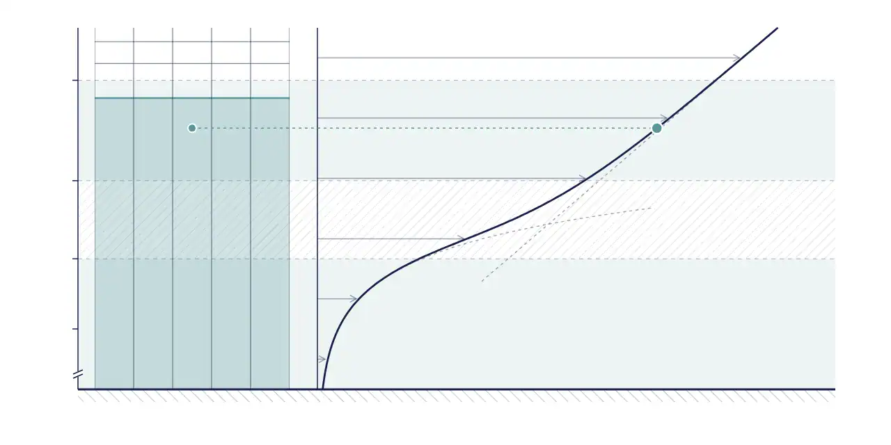
Not every model offers every wall treatment: two-layer k–ε models use Two-Layer All y+, the high-Reynolds Realizable and Standard k–ε offer only High y+, and Spalart-Allmaras offers Low y+ and All y+. Not sure which turbulence model or wall treatment to use? The Turbulence model selector recommends both for your case.
Formulas, assumptions and validity
The calculator estimates the wall shear stress from skin-friction correlations for a smooth flat plate (external flow) or a smooth pipe (internal flow), then solves the definition of y+ for the wall distance. To check the Reynolds number and whether the flow is laminar or turbulent first, use the Reynolds number calculator.
ReL = ρUL / μ (1)
Cf = 0.058 Rex−1/5 (2)
External flow, evaluated at x = L: local skin friction on a smooth, fully turbulent flat plate (Prandtl, 1/7-power velocity profile), about 5 × 10⁵ < Rex < 107.
Cf = 0.079 ReD−1/4 (3)
Internal flow: Blasius, smooth pipe, Fanning friction factor, about 4 × 10³ < ReD < 105.
τw = ½ Cf ρU2 (4)
uτ = √(τw / ρ) (5)
yP = y+μ / (ρuτ), Δy1 = 2yP (6)
δ = 0.37 x Rex−1/5 or δ = 5.0 x Rex−1/2 (7)
Turbulent and laminar flat plate, with Rex = ρUx / μ.
total = Δy1(rn − 1) / (r − 1), last = Δy1rn−1, ratio = rn−1 (8)
For geometric-progression stretching. The terms are shown in the figure above.
Assumptions: a smooth wall, zero pressure gradient, incompressible and steady flow, and a turbulent boundary layer from the leading edge. For external flow the correlation is evaluated at x = L, where the wall shear on a flat plate is lowest, so y+ will be higher further upstream. Treat the result as a starting point and check y+ after your first run.
Worked example: air over a 1 m plate at 20 m/s
Air at 20 °C (ρ = 1.204 kg/m³, μ = 1.813 × 10⁻⁵ Pa·s) flows at 20 m/s over a 1 m flat plate, and the target is y+ = 1. These are the calculator's default values.
ReL = 1.33 × 10⁶, which is inside the range of the turbulent correlation. Cf = 3.46 × 10⁻³ and τw = 0.833 Pa, so uτ = 0.832 m/s. The cell centre must sit at yP = 18.1 µm, which gives a first cell height Δy1 = 36.2 µm.
At x = 1 m the turbulent boundary layer is δ = 22.1 mm thick. Seven prism layers with a stretching of 1.2 grow to 468 µm, and the last layer is 108 µm, about three times the first. Together they cover only about 2 % of δ: the rest of the boundary layer is resolved by the core mesh, so check the transition in step 4, or add layers if you want the prism layer to cover more of it.
Check y+ after your first run
Correlations give a starting value, not the final answer. After the first converged run, plot the Wall Y+ field function on your wall boundaries in a scalar scene. Expect variation: y+ is higher where the flow accelerates and lower near stagnation and separation.
Because y+ scales roughly with the wall distance, rescaling the near-wall thickness by target ÷ actual y+ is a good first approximation; remesh and check again. Once y+ is on target, keep the prism layer settings fixed and refine only the core mesh in a mesh independence study. Our Simcenter STAR-CCM+ training covers meshing and wall treatment in more depth.
References and changelog
References
F. M. White, Fluid Mechanics, 5th ed., McGraw-Hill, 2003: chapter 6 (Blasius pipe friction) and chapter 7 (Prandtl's 1927 flat-plate relations, about 5 × 10⁵ < Re < 107).
H. Schlichting, Boundary-Layer Theory, 7th ed., McGraw-Hill, 1979: chapter XXI (turbulent flat plate at zero pressure gradient, power-law skin friction).
H. Reichardt, “Vollständige Darstellung der turbulenten Geschwindigkeitsverteilung in glatten Leitungen”, ZAMM 31(7), 1951, 208–219: the law-of-the-wall curve in the chart.
Review
Reviewed by Christoffer Johansson, M.Sc., Senior Application Specialist at Volupe. Version 2.1.
Changelog
13 September 2023: the first cell height is reported as the full cell height (2 × the wall distance of the cell centre). Earlier versions reported the cell-centre distance.
October 2026: new interface. Rex is now computed from x (it stayed at ReL when x was edited). Validity warnings added. Same correlations, so default results are unchanged.
November 2026 (version 2.1): solve for the y+ of an existing mesh, boundary layer coverage in step 3, a law-of-the-wall chart of your cells, unit choices and a link that keeps your inputs. The correlations are the same, so default results are unchanged.
November 2026 (version 2.2): the wall-function range and the stretching advice now quote Siemens’ guidance for Simcenter STAR-CCM+ (y+ 30–150 for most cases, stretching 1.1–1.5).
Questions about y+
Calculator reviewed by
Christoffer Johansson
Senior Application Specialist, M.Sc.
Questions about near-wall meshing? We reply within one day.
Ask a technical question →
What is y+ in CFD?
y+ is the dimensionless distance from a wall, y+ = uτy/ν. It tells you which part of the boundary layer the first cell sits in: the viscous sublayer (y+ below about 5), the buffer layer (5–30) or the log layer (about 30–300). Turbulence models treat these regions differently, so the mesh has to match the wall treatment.
What y+ should I use with the k-ω SST model?
SST works with a resolved wall (y+ ≈ 1) or with wall functions (y+ 30–300). Aim for y+ ≈ 1 when wall shear, heat transfer or separation matter. In Simcenter STAR-CCM+ the All y+ Wall Treatment handles both, but avoid leaving most of the wall in the buffer layer.
Is the first cell height the full cell or the distance to the cell centre?
The full cell. Simcenter STAR-CCM+ evaluates Wall Y+ at the centroid of the wall cell, about halfway up a prism-layer cell, so the calculator doubles the wall distance. Since September 2023 it reports the full height, which is the value to enter as the near-wall thickness.
Which length should I use for L?
For external flow, use the length of the body in the flow direction, such as a plate length, chord or vehicle length; for a cylinder or sphere, use the diameter. For internal flow, use the hydraulic diameter Dh = 4A/P and the bulk velocity.
How many prism layers do I need?
Enough to grow smoothly from Δy1 to a size that matches the core mesh. Siemens advises stretching ratios of 1.1–1.5; about 1.1–1.3 is common near walls. Wall-resolved meshes (y+ ≈ 1) need many more layers than wall-function meshes, often 15–30, depending on the stretching and how much of the boundary layer you want the prism layer to cover. Use step 4 to check that the last layer meets the core mesh smoothly.
Why is the y+ in my simulation different from the target?
The calculator uses correlations for a flat plate or a straight pipe. Real geometries accelerate, decelerate and separate the flow, so the wall shear, and with it y+, varies along the wall. For external flow the estimate is made at x = L, where flat-plate wall shear is lowest. Check the Wall Y+ field after the first run and adjust. To see what a given first cell height gives, switch the calculator to “y+ of my mesh”.
Can I use this calculator for Ansys Fluent or OpenFOAM?
Yes. The physics does not depend on the solver. The calculator reports the full height of the first cell for a code that evaluates y+ at the cell centre; if your solver evaluates it at the first node instead, use half that height. Your solver’s documentation says which it is. Only the prism layer setting names are specific to Simcenter STAR-CCM+.