We have seen lately a set of simulations, from different sources, where the coupled implicit solver is used for transient simulation of the type where several species are involved. Either filling or evacuating a tank with one specie, where another is already populated. Like using a higher inlet pressure, in the example, 1 bar gauge, to fill a rigid tank with O2. The tank from the start has 100 % N2 initialized at atmospheric pressure. This is the example we will use in this week’s blog post, and the picture below shows what it looks like, with some measurements and boundary conditions and initial conditions.

The question you could ask yourself in a simulation like this, is how long does it take before we have reached a constant pressure in the tank? Since we have an inlet pressure of 1 bar higher than the initial pressure there is only a matter of time (literally), before the tank is filled with a certain amount of O2, together with the N2 already inside, and the pressure in the tank is also 1 bar, since the inlet pressure in constant.
The way to set this up using default settings can be found in the picture below. Selecting the coupled implicit solver with the implicit unsteady method, you will get the default setting accordingly. A constant CFL of 50 and no “extra” selection like special initialization or CCA.
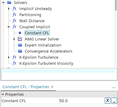
You would run your case with these settings, manually increasing the timestep from a smaller timestep in the beginning – to a larger timestep in the end, to make sure that the simulation runs smoothly. Starting with 1e-4 s for the first iterations, and go towards 1e-2 s or something similar toward the end of the simulation, and you would see the results looking typically like this:
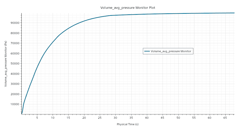
You would theorize that it takes about 60 seconds for the pressure in the domain to reach gaughe pressure, and 90 % of the way is reached in about 18 seconds. And more over, you would be wrong! It is not easy to see, but if this was the only property, except for resuduals you where evaluating during the simulation, you can still spot the error. Early on in the simualtion when we increase the timestep size there are discontinuities in the pressure curve. This is what happens with the curve if we focus on the result in the beginning.
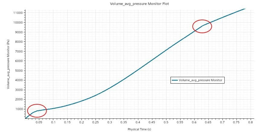
At a couple of different points in time we have discontinuities in the pressure curve. This happened while the time step size was changed. This tells us, already here that we do not have a timestep independent result in our simulation!
If we investigate this further, we can see that something is wrong. For one thing, it is easy to calculate the initial mass in the domain for the N2, either by using the ideal gas law, or simply by initializing the simulation and do a sum-report of density*MassFraction_N2*Volume. The value provided by either of those methods, allow us to know the initial mass, and not only that, but also the mass of N2 at the end of the simulation. There is no N2 leaving the domain, aside from a couple of time steps in the beginning or the near the end of the simulations, where we might have reversed from on the outlet, the only specie passing through in any relevant quantity is O2. Tracking the total mass of either specie in the domain can then give a good sanity check to see if our result can be deemed physical. The Total mass of N2 should not change as no N2 is leaving via the inlet.
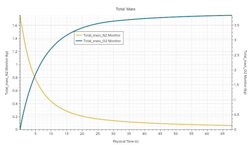
Looking at the plot to track these quantities, we can see that the mass of N2 does not at all behave the way we would expect, it rather seems like when we push in O2 we also push out N2. Conclusion here is that the result is wrong, and the simulation cannot be trusted. Later we will see similar representations where the results from several different simulations are put in the same plot, but some crucial settings have been changed. But first we need to understand what is going on here. Why does this happen, and how can we prevent it?
CFL number
A short mention of the CFL number was given in my latest blog post about being pragmatic when solving your CFD simulations, it can be found here [Solving the engineering question – VOLUPE Software]. There it is stated that the CFL number setting for the coupled solver is what is used to decide the pseudo-timestep for the coupled solver. The CFL number should be seen as a under relaxation factor for the coupled solver, meaning that small numbers will hopefully increase the stability of the simulation, at the cost of more iterations to reach convergence. This becomes extra intricate in a transient simulation, because here we essentially have a dual-timestep method. The Implicit Time stepping, or Dual Time-Stepping is the one transient method that we will focus on here. The other method is the Explicit Time-Stepping method, in which you specify CFL number that is used to set the physical time-step for all cells in the domain. This is rarely used in Simcenter STAR-CCM+ because it is very time consuming but is used in many other numerical methods. We are not going to focus on the mathematics here for brevity, but in the Implicit time-stepping, we use the dual time-stepping, with inner iterations in pseudo-time. This means that as well as getting a timestep independent solution for any transient simulation, we need to make sure that the simulation is timestep independent both in terms of the global timestep and the pseudo timestep. And this is what is happening in the simulation above looking at the mean pressure in time. When we change (increase) the global timestep at those highlighted locations, we reduce the slope of the curve, meaning that the goal, when we reach equilibrium pressure, is pushed ahead of us in time. And as stated previously, we do not have a time-independent solution.
CCA
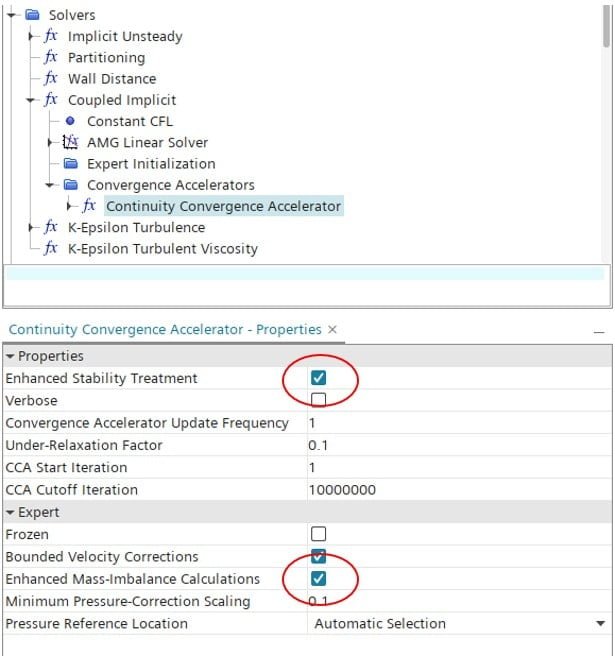
The dual time-stepping issue here is one side of the coin, and the other one is the poor result for the mass. This can be attributed to the lack of CCA and solved with the inclusion of CCA. The CCA stands for Continuity Convergence accelerator and is a method that can be applied to the coupled solver. There is a blog post on the topic written by Christoffer that partially explain the CCA, Coupled solver settings in Simcenter STAR-CCM+ – VOLUPE Software. In short it is a tool that can be used when convergence of mass balance is slow. And this is exactly what we have seen in simulations with several species. Meaning that we have large improvements in mass balance and continuity when using the CCA. It should be used with Enhanced stability treatment and with Enhanced Mass-imbalance Calculations activated for the best result.
Improving on the initial simulation
We have now identified the issues and also understood how we can improve the simulation in order to obtain results that we can trust. For this type of simulation, we can then test what impact the CFL number and the use of CCA have on the result. The testing has been limited to these two settings and the values used for CFL is 50, which is default in star, and “Automatic”, where the solver decides. For now, it is good to understand that in practice means orders of magnitude larger than the default value. And the CCA has the option of being on, with the above-mentioned tick-boxes, or off. The segregated solver has also been used for reference. The first curve we looked at here is the blue one, and it is by far the longest estimation of reaching equilibrium conditions. We can se that with the inclusion of the CCA for the CFL 50, we get a better result, but far from optimal. It is when we allow for the higher CFL number that the results is the same. And in this case, we see that we reach equilibrium in about 4 seconds, compared to the 65 seconds shown in the first simulation. In this particular case, the Automatic CFL did not also “need” the CCA to reach the same result, but with a poor CFL, the CCA helped in the right direction.

If we instead look at the total mass, we see that with the low CFL and no CCA, after the simulation is done, we have no N2 left in the tank. In the simulation it seems like the O2 has replaced the N2, something that cannot happen in reality of course. In both simulations with CFL auto, the mass N2 is preserved.

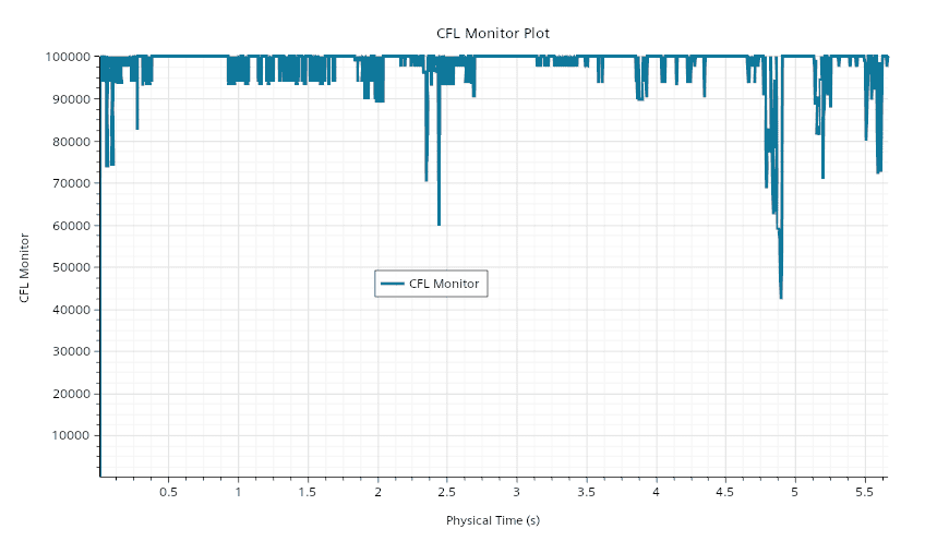
For reference we also look at the CFL plot along the time in the Simulation with Automatic CFL including CCA and see that the value is almost always maxing out at 1e5. (There is a limit even for the automatic setting, saying CFL min 0.1 and max 100000.)
Conclusion
From this we bring the conclusion that a CFL number which is as high as possible should be used, together with the CCA for thorough mass balancing of the simulation. We also bring with us the need to look at several properties and details of the simulation to make sure that what we get makes sense and is correct.
Best practice template for this type of coupled flow
This file can be obtained from the CFD handbook part of the volume homepage as a best practice template on the Volupe best practice side. [Templates – VOLUPE Software]
I hope you can use this and that this has been a learning experience. All details regarding both CFL and CCA can be found in the documentation. Ans as usual, reach out to support@volupe.com with any questions.
Author

Robin Victor
+46731473121
support@volupe.com