In this week’s blog post we will extend our prowess into the combustion modeling options we have in Simcenter STAR-CCM+. Last time we looked at the options for reacting species transport, the EBU and complex chemistry variations [Combustion In Simcenter STAR-CCM+, Reacting Species Transport – Volupe.com]. This time we will look at Flamelet based modeling and its variations.

Before the deep-dive into the variations we need to understand what the flamelet based models do and how they work, there are a few central terms that we need to understand in order for this to make sense. Note that the flamelet based models can much more easily handle a larger number of components and reactions. We do not track individual species but break the system into flamelet tables used instead. This will be apparent when describing the central terms.

Instead of simulating all species, as we would typically do in reactive species transport, we can use flamelet modeling to reduce the system down to a chemical state space. A laminar flamelet is a mathematical model for turbulent combustion and is specifically formulated to deal with non-pre-mixed combustion. The concept considers the turbulent flame as an aggregate of thin, laminar, locally one-dimensional flamelet structure existing in the turbulent flow field. The chemical state space is tabulated using pre-computed tables to store the information. We then use, 3 or 4 (depending on the model selected) parametrized variables that are transported during the simulation. The most common such variables are Mixture fraction, Heat loss and Progress variable.

Mixture Fraction

One of the large strengths of the Flamelet models is use of parametrizable variables, where the mixture fraction is the elemental mass fraction that originated from the fuel stream. It is a conserved scalar with the value 1 for the fuel stream and 0 for the oxidizer stream. For the flamelet method the transport equations are solved for the mixture fraction and use that to obtain the species mass fractions. It is calculated using:

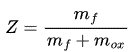
Where, m_f is the total mass of all elements that originate from the fuel stream at any spatial location and m_ox is the total mass of all elements originating from the oxidizer stream.

The mixture fraction variance is another parameter used in FGM (Flamelet generated manifold) simulation, used to account for the effect of turbulence on the combustion taking place. It is calculated based on the turbulence fluctuations of the mixture fraction and it is used to modify the laminar flamelet library to account for the effects of turbulence.

Progress variable

The progress variable indicates a thin layer that divides the calculation domain into unburnt and fully burnt, with the intermediate zone in between. By this definition in each cell, we can solve for a transport equation that tracks the progress of the transition between unburnt to fully burnt states. The progress variable c is between 0 and 1, where 0 is unburnt and 1 is fully burnt. Its source term differs depending on the specific combustion model.

Flamelet models

In this section we will go over the different flamelet models, both when they are valid and also what limitations they might have.

The chemical equilibrium model

The chemical equilibrium model assumes that what is mixed has also reacted and reached chemical equilibrium. The equilibrium state is computed by minimization of the Gibbs free energy. It also makes the simplification that all species diffuse at the same rate, an assumption valid for turbulent flow where the turbulent diffusivity is much higher than the molecular diffusivity. Other than tracking the mixture fraction and its variance described above, we also solve for heat loss ratio. The heat loss ratio is used to indicate the amount of heat loss or gain. It represents the departure of the system from its adiabatic state.

The chemical equilibrium model can be used when no kinetic mechanism is available, meaning that it still requires the reaction to be setup, but it does not require the stoichiometry or any Arrhenius parameters or chemkin data respectively. This is solved instead by minimizing the Gibbs Free energy. It can be used when chemistry is considered fast relative to the mixing and when there are no ignition and extinction events or other complex flame dynamics like lift-off.

SLF

In the steady laminar flamelet we consider the turbulent flame an ensemble of laminar flamelets where the chemical reactions occur in thin zones. We assume that the zone is thinner than the size of the Kolmogorov scale. If there are eddies that can penetrate the reaction zone flamelet, this assumption is no longer valid.

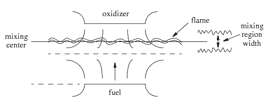
The underlying mechanisms are solved by interpolating from tables, and we use steady flamelet equations to solve for the table being generated. We use the variable Mixture fraction and scalar dissipation rate to describe the chemical state space. The scalar dissipation rate is modeled as:

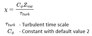
The flame temperature is strongly dependent on scalar dissipation rate. The maximum flame temperature decreases with increasing scalar dissipation, meaning that high values of scalar dissipation can lead to extinction. At a scalar a dissipation value of zero, the flamelet is at chemical equilibrium. Variables solved for are all expressed as functions of the scalar dissipation rate, the mixture fraction, and the heat loss ratio (the enthalpy).

FGM

The flamelet generated manifold differs from the chemical equilibrium and SLF in that the mixture fraction is included in the parametrization of the thermo-chemistry. We can use a 0D constant pressure reactor or a 1D premixed flamelet to generate the FGM manifolds. The variables of interest for tabulation are the mixture fraction, its variance, heat loss ratio, the progress variable and its variance. The FGM model is appropriate to model premixed and partially-premixed flames.

In the 0D constant pressure reactor, during the tabulation process we solve the following equations for mixture fraction and heat loss ratio:

This is a purely kinetically controlled system, meaning that we can capture kinetically controlled phenomena such as lift-off.

For the 1D premixed flamelet, we solve the following opposed-flow premixed equations in progress variable space at a fixed mixture fraction, assuming unity Lewis number:

The equations are integrated in pseudo-time until the unsteady terms on the left-hand side are small. The residual is defined as the sum of the normalized absolute values of the unsteady terms over all points, for temperature and post-processing species. The equations are considered converged when this residual is less than the specified Flamelet Convergence Tolerance parameter.

There are three different methods for calculation of the progress variable for FGM. The first one, the FGM Kinetic Rate, calculates the source term from the chemical kinetic reaction rate, interpolating from the FGM table. The Coherent Flame Model (CFM) assumes that combustion occurs in the flamelet region. The mean turbulent reaction rate can be expressed as the product of the flame surface density, the laminar flame speed, and the unburnt density. A transport equation is solved for the flame surface density. The Turbulent Flame Speed Closure (TFC) assumes that in a premixed combustion system, the reaction takes place in a thin layer which separates reactants and products. The mean reaction rate is closed using the turbulent flame speed.

Reference case – Sandia Flame

As in the previous post, the Sandia flame is used as a reference, and as a reminder: In the simulation the geometry is a two-dimensional axisymmetric geometry consisting of the main jet nozzle and the pilot jet inlet. It burns a pre-mixture of 25% methane and 75% dry air by volume. It is shown in the picture below.

For the chemical equilibrium model we use a Non-adiabatic PPDF Equilibrium, Realizable K-Epsilon and a Two-Layer All-y+ Wall Treatment. And the results are presented below.

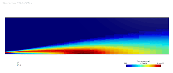
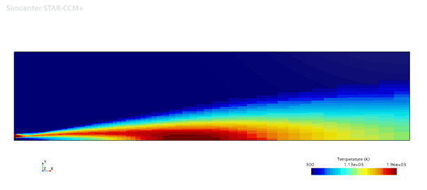
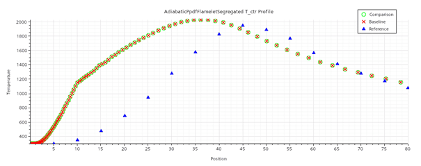
The flamelet model is simulated using the same turbulence settings with FGM kinetic rate, FGM reaction, Gray DOM radiation and the results are shown below.

I hope this blog post has been useful and informative to read. Remember that there are loads of information pertaining to the models in the Simcenter STAR-CCM+ documentation. One thing that has not been brought up in any of the two chemistry/combustion posts is the emission models that are available. You can simulate NOx and soot formation, usually as sort of a post processing step. Please see the documentation for further information. If there are any questions reach out to support@volupe.com.

Author

Robin Victor
+46731473121
support@volupe.com