Time-step selection in a conjugate heat transfer analysis

Johan BernanderSenior Application Specialist
Selecting a time-step size in a transient simulation is a matter of assessing how fast you can progress the solution while still being time-accurate. In other words, how fast can you progress while still capturing all relevant physical phenomena. In many transient CFD analyses, the solution progression is typically limited by the transient evolution of fluid flow. But in a conjugate heat transfer analysis, there may be cases where the thermal transient within a solid evolves faster than the flow field, particularly when highly conductive materials such as aluminum or copper are involved. In this article, we will describe what measures you can use to assess the limiting physics for the time-step selection in conjugate heat transfer.
Characteristic time scales
To assure a time-accurate solution of a physical problem, the time progression must resolve the shortest characteristic time scale of the relevant physics, and different physical phenomena have different characteristic time scales.
The characteristic time scale for fluid flow, t_{flow}, is the time required for a fluid to travel a characteristic length, and can be simply defined as
t_{flow}=\cfrac{L}{U}
where L is the characteristic length and U is the characteristic fluid velocity.
Similarly, the characteristic time scale for solid conduction (or diffusion), t_{diff}, is the time required for heat to diffuse over a characteristic distance, typically defined as
t_{diff}=\cfrac{L^2}{\alpha}
where L is the characteristic length and \alpha=k / \rho c_p is the thermal diffusivity of the solid. Substituting the thermal diffusivity, the diffusive time scale can instead be expressed as
t_{diff}=\cfrac{\rho c_p L^2}{k}
where \rho is the solid density, c_p is the specific heat and k is the solid thermal conductivity. This formulation is sometimes more approachable in terms of material parameters.
The Courant number and the Fourier number
Tightly connected to the characteristic time scales are the non-dimensionalized versions of the same: the Courant-Friedrichs-Lewy (CFL, or sometimes simply Courant) number and the Fourier (Fo) number. While the characteristic time scales indicate the overall evolution time of the physical phenomenon, the Courant and Fourier numbers relate to the discretization requirements for time-accuracy of the numerical formulation of the physical problem. In other words, they take time-step and mesh resolution into account.
For fluid flow, the CFL number provides the relevant criterion for determining the required time-step size, given the local mesh conditions. The CFL number is defined as
CFL=\cfrac{\Delta t}{t_{flow,local}}=\cfrac{u \Delta t}{\Delta x}
where u is the local fluid velocity, \Delta t is the time-step size and \Delta x is the spatial grid size. As such, the CFL number relates the time-step size to the local flow time scale,
t_{flow,local}=\cfrac{\Delta x}{u}
i.e. the evolution time of flow through a finite volume cell.
A CFL number of 1 means that the fluid flow traverses one full cell in one time-step. Hence, the general recommendation for a time-accurate flow simulation is to keep the CFL number below or equal to 1. For explicit time integration this is even a stability requirement for the solution algorithm, while implicit time integration can handle larger values. Transient simulations in Simcenter STAR-CCM+ generally implement implicit time integration, meaning that the CFL number will mainly dictate the time-accuracy of the solution progression, and not necessarily crash if the condition (CFL ≤ 1) is not met.
For thermal conduction/diffusion, the Fourier number provides the relevant criterion for determining the required time-step size, based on the local mesh conditions. The Fourier number is defined as
Fo=\cfrac{\Delta t}{t_{diff,local}}=\cfrac{\alpha \Delta t}{\Delta x^2}=\cfrac{k \Delta t}{\rho c_p \Delta x^2}
hence relating the time-step size, , to the local thermal diffusive time scale,
t_{diff,local}=\cfrac{\rho c_p \Delta x^2}{k}
i.e. the time it takes for heat to diffuse across one finite volume cell. For explicit time integration, the limit for the Fourier number scales with solution dimension, such that
Fo \le \cfrac{1}{2n}
where n is the dimension of the problem. This means that for a 1D simulation, the Fourier number must oblige Fo \le 1/2, for a 2D simulation Fo \le 1/4 and for a 3D simulation Fo \le 1/6 to be conditionally stable. For implicit time integration, which is typically the case in Simcenter STAR-CCM+, the requirement is less strict since the time discretization scheme is unconditionally stable. This means that, similarly to the CFL, the Fourier number will mainly dictate the time-accuracy of the solution progression and not necessarily the solver stability. As a rule of thumb, it is usually acceptable to aim for a Fourier number in the order of unity or less.
Finding the limiting factor
Let’s look at an example to concretize the reasoning and find the limiting factor for a specific problem. Consider a hot aluminum block of 0.01 meter in thickness, that is cooled on a 0.1 meter high side by a natural convection fluid flow of 0.02 m/s.
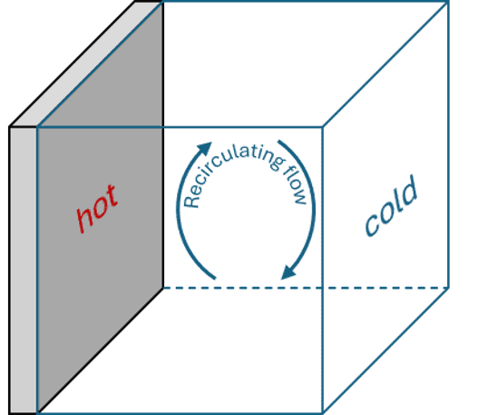
The characteristic fluid time scale for that case would be
t_{flow}=\cfrac{0.1}{0.02}=5 s.
The aluminum has a density of 2702 kg/m3, a specific heat of 903 J/kg-K and a thermal conductivity of 237 W/m-K, giving a characteristic diffusive time scale of
t_{diff}=\cfrac{2702 \cdot 903 \cdot 0.01^2}{237} \approx 1.03 s.
Comparing these two characteristic time scales, one can see that the thermal transient in the solid can be expected to evolve almost five times faster than the fluid flow. Note that for the diffusive time scale, the 0.01 meter thickness of the aluminum block was chosen as the characteristic length, assuming that the thermal gradient of interest would be through the thickness of the block.
Now, let’s take the spatial discretization into account and look at the Courant and Fourier numbers. For simplicity, let’s assume we have used a uniform, equidistant hexahedral mesh size of 5 millimeters. Moreover, we want to maintain CFL=1 and Fo=1. This gives us the following limits for the time-step size:
\Delta t_{flow}=\cfrac{\Delta x}{u}\cdot CFL=\cfrac{0.005}{0.02}\cdot 1=0.25 s
\Delta t_{diff}=\cfrac{\rho c_p \Delta x^2}{k}\cdot Fo=\cfrac{2702 \cdot 903 \cdot 0.005^2}{237}\cdot 1 \approx 0.26 s.
So, given the current mesh resolution and physical behavior, the required time-step for a time-accurate simulation is coincidentally the same for both the fluid and the solid. This is, of course, usually not the case and obviously highly dependent on the spatial resolution (and the solid material properties). Let’s say we would have used a cell size of 2.5 millimeters instead – then the time-step limits would have been:
\Delta t_{flow}=\cfrac{\Delta x}{u}\cdot CFL=\cfrac{0.0025}{0.02}\cdot 1=0.125 s
\Delta t_{diff}=\cfrac{\rho c_p \Delta x^2}{k}\cdot Fo=\cfrac{2702 \cdot 903 \cdot 0.0025^2}{237}\cdot 1 \approx 0.064 s.
In other words, that type of mesh would put higher restraints on the time resolution of the solid conduction. Similarly, if the solid block would have been made of copper instead of aluminum, the diffusive time scale (with the original mesh size) would reduce to
\Delta t_{diff}=\cfrac{\rho c_p \Delta x^2}{k}\cdot Fo=\cfrac{8940 \cdot 386 \cdot 0.005^2}{398}\cdot 1 \approx 0.22 s
which is slightly faster than both the aluminum block (and the flow evolution).
To conclude, the required time-step size for your simulation should oblige
\Delta t=\rm{min}\left(\mathit{\Delta t_{flow},\Delta t_{diff}}\right).
Consequently, while transient CFD simulations are often associated with CFL-based time-step selection, conjugate heat transfer simulations involving highly conductive solids and/or fine meshes may instead be governed by the Fourier-number requirement.