In this week’s blog post we will look into simulations including several phases within Simcenter FLOEFD. We have the opportunity to model both subdomains with different fluids as well as Free surface simulations. The meaning of subdomains is domains with a wall dividing your computational domain into several domains, having the possibility to use different fluids in each subdomain. While free surface will track an interface between two phases in the same computational domain. Free surface simulations are similar to Volume of Fluid (VOF) simulations in Simcenter STAR-CCM+.
Example – Subdomains in a ball valve
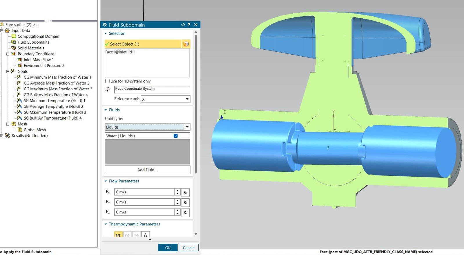
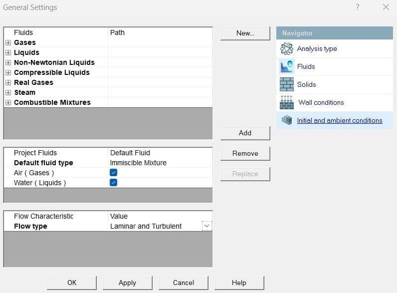
In Simcenter FLOEFD you select a default fluid in your general settings, let’s say you select air for an external simulation of your ball valve. In this example you are interested in the heat transfer in the air, where the temperature of the ball valve will be dependent on the warm water that flows inside. To include a new fluid, you add it in the general settings and keep air as the default fluid – we will use water as our second fluid. In the tree-structure you right-click on the Fluid subdomain folder to include your second fluid. By selecting which type of fluid (sorted based on phase, in this case liquid) you can specify water and select a surface to decide which cavity should be used as subdomain. See the picture below where the fluid subdomain is visualized. When this is completed, you can specify your boundary conditions for your computational domain. You will now have a natural convection simulation with air, around a ball valve with water inside, where solids act as walls between the fluids and heat can be transported in all media.
Example – Free surface simulation inside a ball valve
If we instead want to have air in the ball valve as initial condition, and then let warm water flow into this part of the domain we can use Free surface instead of Fluid subdomains. In general settings you can activate Free surface by ticking in the Free surface model in Analysis type. In the Fluids tab, see picture below, you can then add immiscible fluids (an immiscible mixture) like in our case of air and water. Immiscible means that these two fluids will not mix.
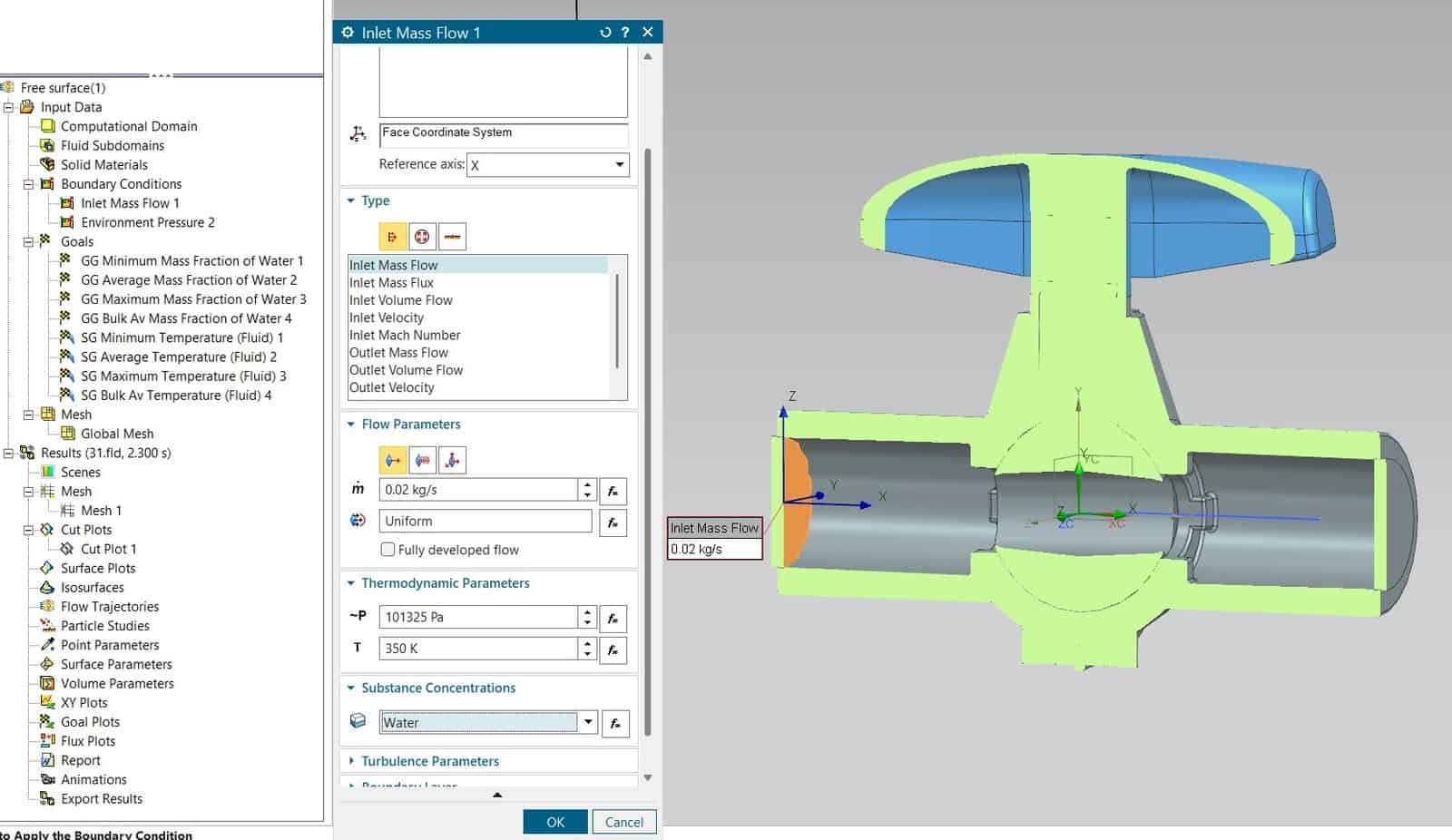
As boundary condition for the fluid inlet, you now add the Substance concentration, which in this case should be water. This will allow you to start with air in both the external domain and inside the ball valve, and the water will push out the air and fill the internal domain. If you would like to use a table/function for defining a varying concentration of fluid as boundary condition, there is availability for that as well. As usual, you specify all boundary conditions at the internal wall that you want the fluid to flow in from.
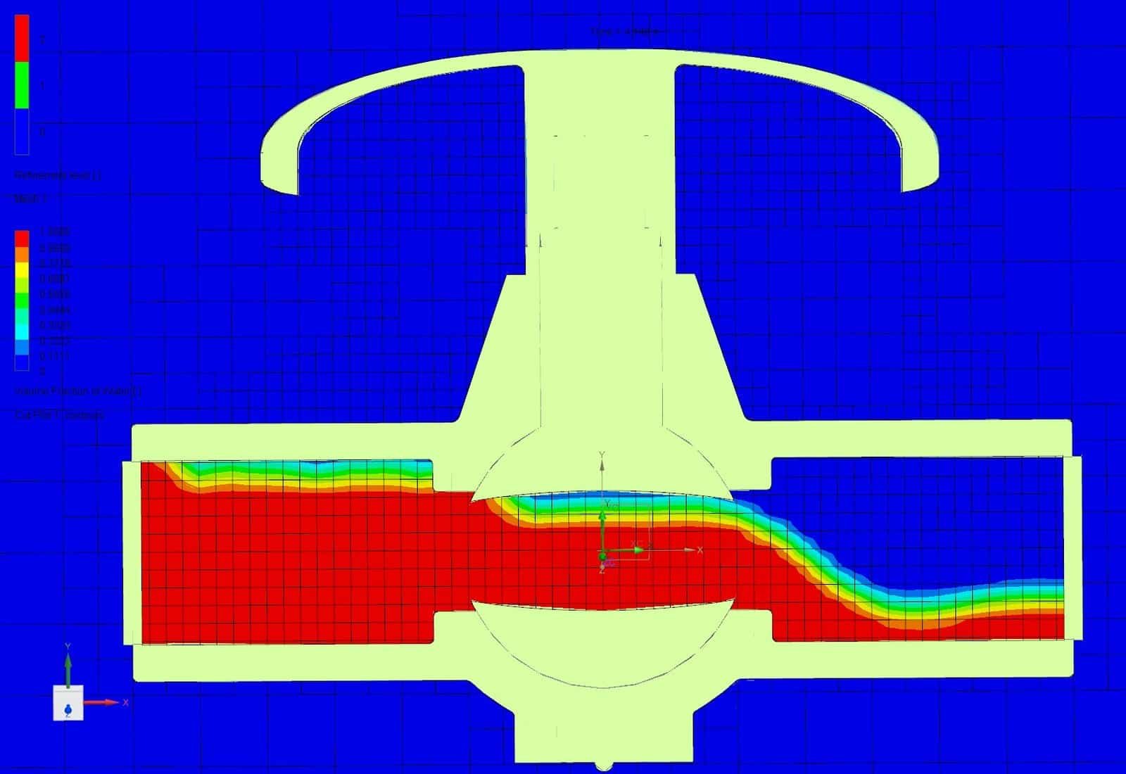
Depending on how much water you set as inlet boundary flow condition you will fill up the domain to a certain level. In the picture below you see the solution for this example, where the mass flow is low enough to not push out all the air. The colors indicate the level of water volume fraction, where red is 1 (100% water) and blue is zero (100% air). The water goes into the internal domain from the left and flows out to the right. The grid in the picture is displayed to represent the mesh resolution. The global mesh size is set to level 5 of out 7, providing a coarse mesh as reference to the refined examples further down.
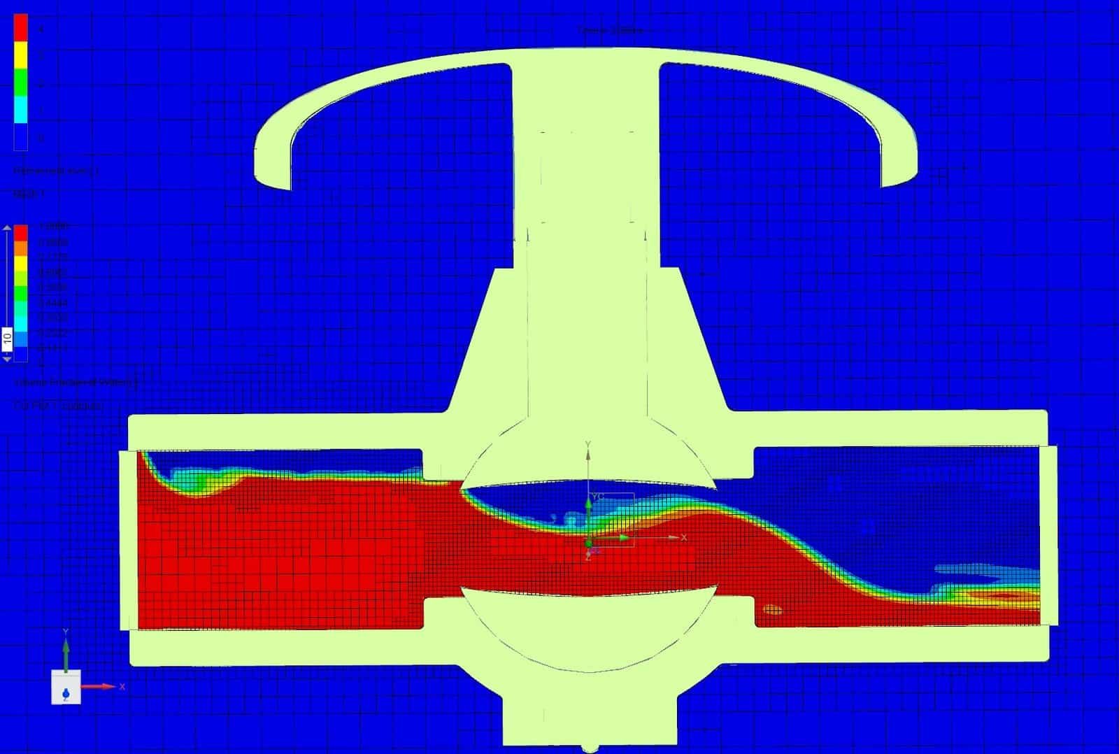
To resolve the water surface to a finer level you can combine your free surface simulation with Solution-adaptive meshing (also known as AMR), as we discussed in a recent blog post at the Volupe blog, see https://volupe.com/simcenter-floefd/solution-adaptive-meshing-in-simcenter-floefd/. In the picture below, you see what a very fine mesh can look like for this simulation. Allowing the cells to be refined to an additional level after level 7 for the global mesh you really see that the finer cells are located close to the free surface, and the walls, where gradients are high to volume fraction and velocity. The level of detail in the flow field is much higher than in the simulation using level 5 mesh, where the free surface instead is smeared out.
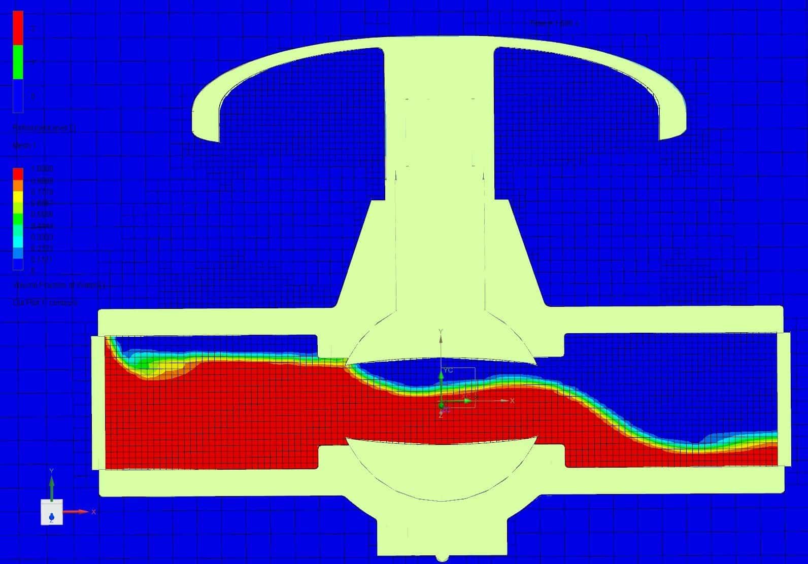
AMR can save a lot of cells and computational time when you are looking for accurate results but don’t want to have finer cells in the whole domain. So to compare the reference simulation with level 5 mesh, using around 47’000 cells, you will find two more simulation results below. If level 7 mesh is used in the whole domain, as in the first picture below, you end up with around 274’000 cells, providing a fine mesh resolution.
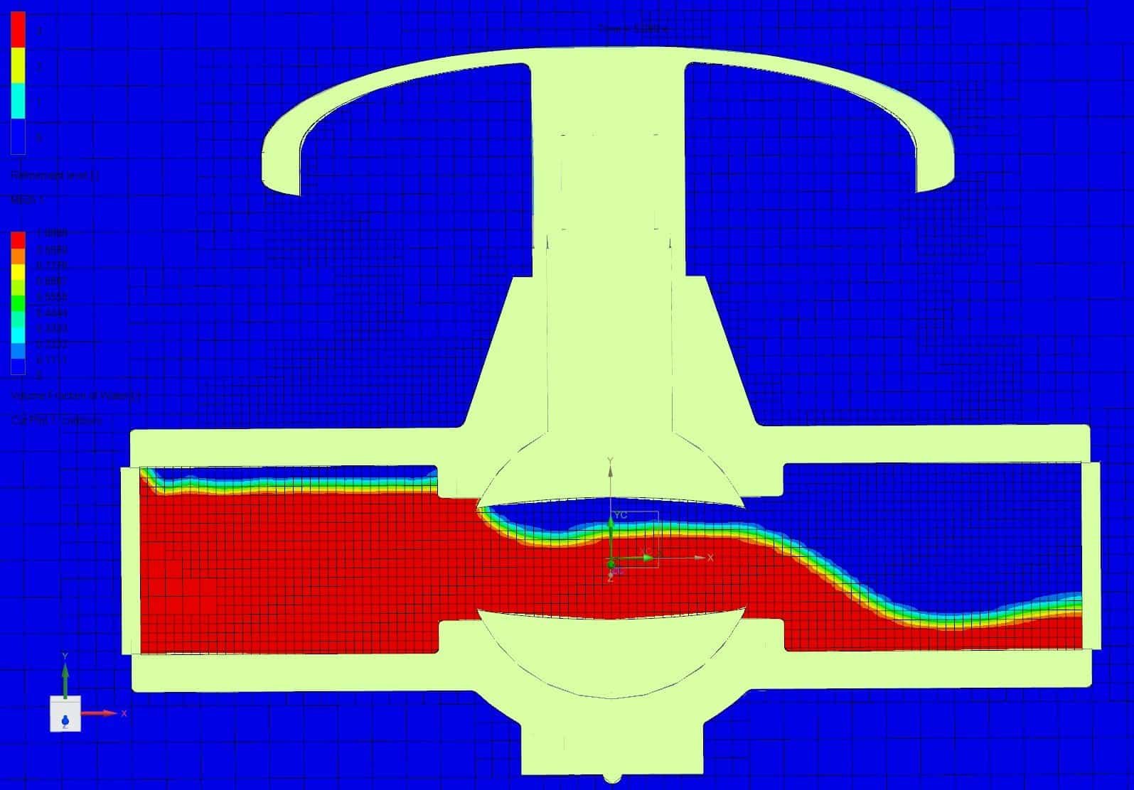
When using AMR to only use finer cells where the gradients are needed, you obtain the mesh resolution visualized below. Here, the number of cells is around 153’000, which is almost half of the number of cells used if level 7 mesh is used in the whole domain. This proves that you can save computational power using AMR, even though you have to consider that the remeshing procedure takes some computational power as well.
Note: The example simulation is run with time-dependency activated, which makes the result differ a bit when it comes to the flow field. The aim of this blog post is to focus on the mesh resolutions, level of detail and over-all flow structure when it comes to the results. Free surface simulations require the solver to be time dependent.
Thank you for reading this blog post about how to simulate combinations of fluids in the same simulation in Simcenter FLOEFD. Hopefully these tips will help you in your every-day simulations and don’t forget that Free surface simulations and Solution-adaptive meshing is a good combination. If you have any questions about your simulations, feel free to reach out to support@volupe.com.
Author
Christoffer Johansson, M.Sc.
support@volupe.com
+46764479945