In Conjugate Heat Transfer (CHT) or Fluid-Structure Interaction (FSI) simulations, thin structures can pose a real challenge when it comes to meshing, typically requiring a very fine surface mesh to uphold a decent mesh quality and provide enough resolution in the normal direction. In this week’s blog post we will demonstrate how you can overcome this and reduce computational efforts using the Thin Mesher algorithm, or even Shell elements, for very thin structures.
Heat transfer through metal sheets
To compare the different methods we will look at a simple example of heat transfer through a number of joint metal sheets. The full geometry consists of four horizontal metal sheets, joint together by a vertical metal sheet. The thickness of each sheet is two millimeters. Below is a depiction of the geometry.
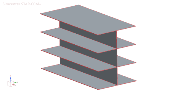
The back end (negative X) of the sheets are given a fixed temperature condition of 50°C, and the front end is given a fixed temperature condition of 4°C. The remaining faces are given a convective boundary condition of 4 W/m-K and 15°C, as if the internals were confined between the hot side and the cold side. The exact values are really of less importance for the comparison, but are included for the sake of completeness.
The reference setup
The standard approach typically used in a general CHT simulation would be to apply an Automated Mesh operation, so this will be the basis for our reference setup as well. In this case we use the Polyhedral Mesher, but the underlying challenge would be similar for the Trimmed Cell Mesher as well. The challenge with the standard meshing approach for this type of thin structures is the need for a fine surface mesh resolution, in order to fit decent quality cells in the solids. In the mesher algorithms, this is typically handled automatically through the “Perform Proximity Refinement” setting (which is always activated as default) in the Surface Remesher.
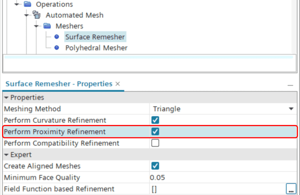
Please note that for this to work properly, the Minimum Surface Size in the Default Controls obviously needs to be small enough. In this case we use the default value, which is always 10% of the Base Size. The Base Size chosen for the metal sheets is 0.005 meters, meaning the Minimum Surface Size will be 0.5 millimeters. The Target Size is set to 200% of the Base Size (although this will not come to use here because of the proximity refinement). The resulting mesh ends up at about 1.8 million cells, with more than 99% of the cells above 0.1 in cell quality. Below you can see a depiction of the mesh.
The Thin Mesher setup
Now, since this analysis would purely involve solid conduction, it’s fair to say that the mesh resolution given by the standard Automated Mesh algorithm is way beyond what would be required for a good result. So, let’s see how we can utilize the Thin Mesher to provide a more efficient setup.
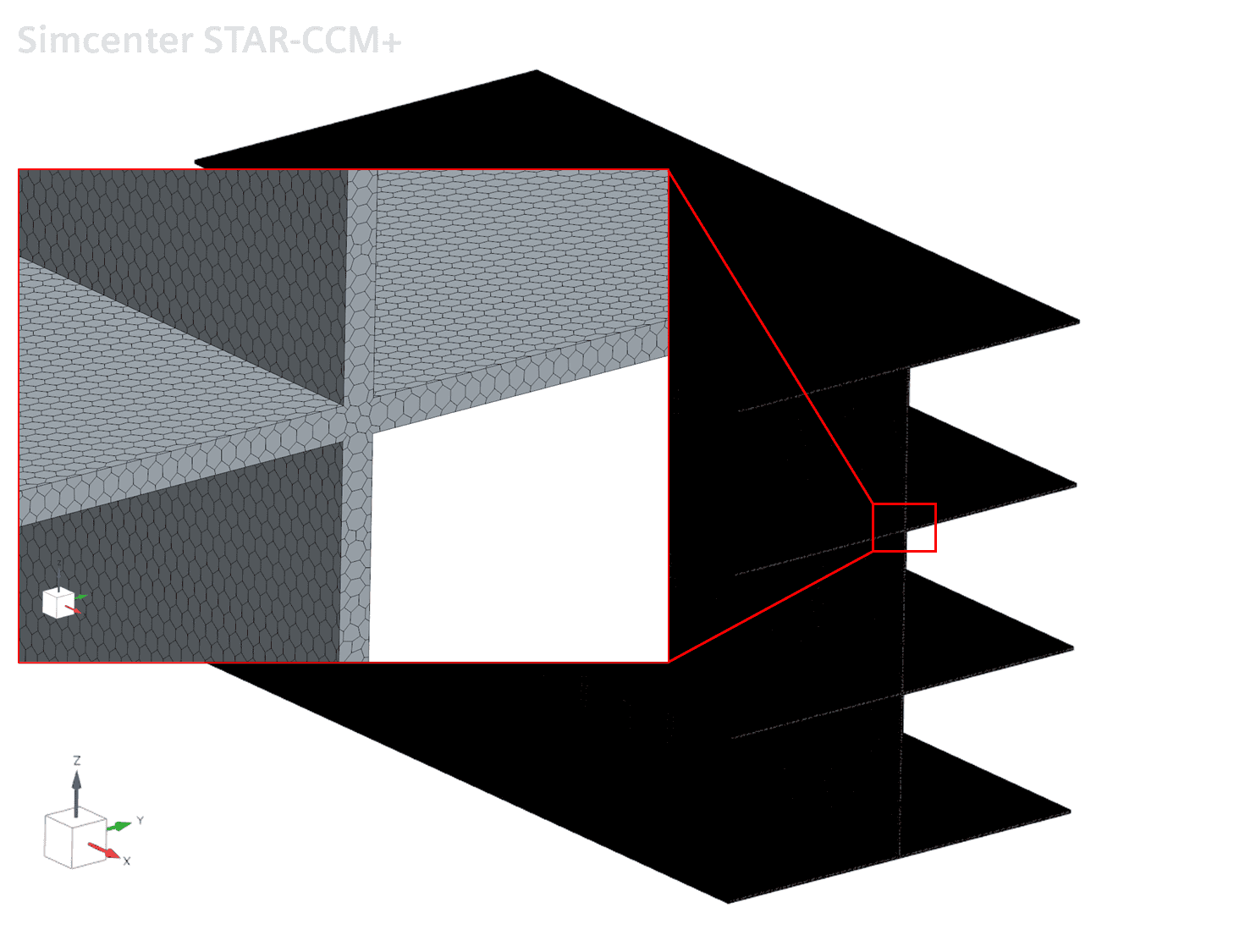
Since the Thin Mesher generates prismatic cells, we can allow the surface mesh size to increase, while still maintaining a decent cell quality within the solids. To do so, we can deselect the “Perform Proximity Refinement” setting for the Surface Remesher. We keep the Base Size (0.005 meters) and Target Size (200% of Base Size) as is and set the Number of Thin Layers to 2. Using this approach, we end up with a mesh that has about 15,000 cells (i.e. less than 1% of the standard mesh) and about 97% of the cells above 0.1 in cell quality. A picture of the resulting mesh can be seen below. As you may notice, the Thin Mesher does generate some irregularities in the joint between the top plate and the vertical plate. However, these irregularities are not necessarily of bad quality and will not cause any problems for the simulation.

The Shell element setup
Yet another alternative that can be useful when you’re working with thin structures is Shell elements. In contrast to the standard and thin mesher approaches, shell elements are two-dimensional, meaning they have no geometric thickness. Instead they are given a purely numerical thickness (defined on region level).
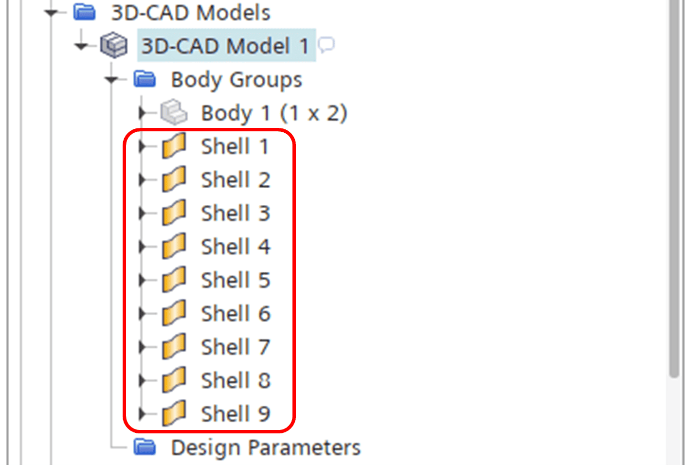
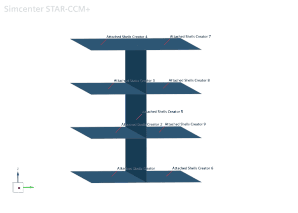
To create such zero-thickness shell elements, the geometry is reworked so that it is built up by nine sheet bodies (rather than one unified solid body): eight horizontal sheets and one vertical. In this case that was done by creating a mid surface in all the solid sheets in 3D-CAD, which were all treated as a separate sheet body.
Once imported into STAR-CCM+ main GUI, the shells are created with the Attached Shells Creator operation.
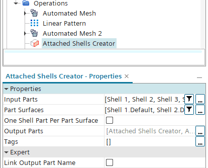
This operation gives us nine new shell parts:
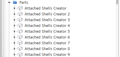
Here you can see them visualized as well:
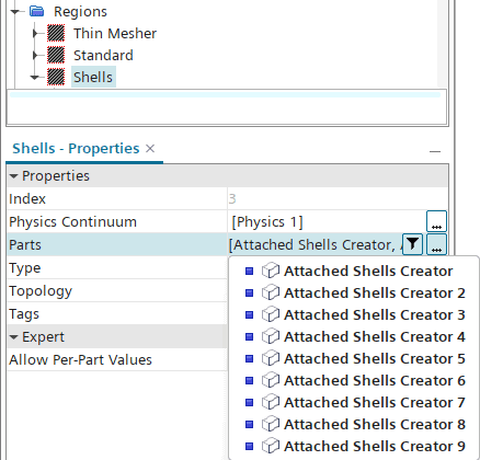
These shell parts are now the ones that are used as input to our shell region, see below:
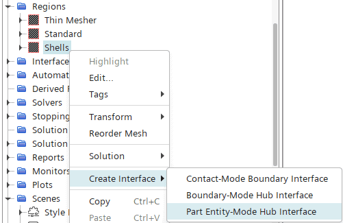
For the heat transfer to work between all the shells, we also need to setup a so-called Hub interface. The Hub interface is an interface that handles interaction between shell edges and other entities (such as other shell edges, shell surfaces or solid surfaces). To create the Hub interface, we right-click the shell region and select Create Interface -> Part Entity-Mode Hub Interface.
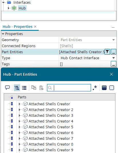
Then our Attached Shells are added as input to the Hub interface, see below:
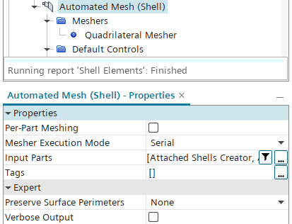
Now we are ready to mesh our shell region, and to do so we use the purpose-made Automated Mesh (Shell) operation. The Automated Mesh (Shell) operation does not support polyhedral elements – it can only produce triangular or quadrilateral shells elements. In this case we chose to go for the quadrilateral mesher.
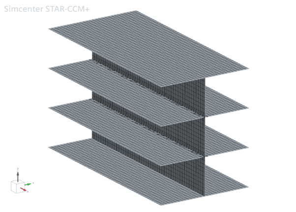
The final shell mesh is shown below, with a total amount of elements of around 7,500. The cell quality metric used for the finite volumes above does not apply to shell elements, but all elements in the shell mesh fall below 60° in skewness angle. Typically, an element is considered bad if the skewness angle lies above 85°.
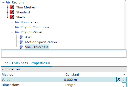
Lastly, the shell elements need to be given a thickness. As mentioned above, this is done inside the region – and more specifically inside the Physics Values folder.
Now we are ready to run a simulation also with shell elements.
Comparing the setups
As outlined above, the different approaches generate widely different amounts of cells/elements. So, how do the results compare to each other? And what about convergence rate? Let’s take a look at the temperature fields for each approach, along with a comparison of the heat balance convergence rate.
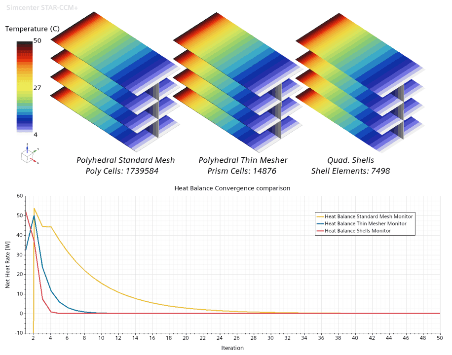
As indicated above, the temperature fields are close to identical for each approach. This is quite expected, since we are dealing with pure thermal conduction here. So, what about the convergence rate? As you can see in the plot, the Thin Mesher and Shell element approaches clearly outperform the standard polyhedral mesh approach. The Shell element setup is more or less converged in just five iterations, and the Thin Mesher setup in about twice as many. The standard approach, however, requires at least 40 or even 50 iterations to reach the same level of convergence, i.e. between 8-10 times slower than the Shell element approach.
One last thing to bear in mind is that if you would like to resolve (and therefore mesh) the surrounding fluid (which we emulated with a convective boundary condition), the shell element approach could pose a challenge if the mesh has to interconnect around the edges of the structure, similar to a mesh with baffles. In a case like that, the Thin Mesher would be the ultimate compromise.
I hope that this comparison has showcased in a good way how you can simplify your thin structures to save computational efforts. As always, you are welcome to send in any questions or comments to support@volupe.com.
Author

Johan Bernander, M.Sc.