In this week’s blog post we will take a look at the multiphase modelling capabilities in Simcenter STAR-CCM+. Seeing as one of the overall strengths in Simcenter STAR-CCM+ is its wide multiphysics and multiphase possibilities, it is of importance to the users of the software to be aware of these possibilities. Not only that, but it is also of great interest for us at Volupe as provider and supporting body of the software, that our clients, current and future, know what is possible to simulate.
It is important to understand the division between “multiphase” from “multi-component”. They are diametrically opposite when speaking of mixing scale. While the multiphase simulations try to simulate and resolve the interaction between your phases, the multi-component flow is already mixed on a molecular level. Meaning that the multi-component flow is seen as one phase since the mixing scale is usually too small to resolve in a CFD simulation. You can of course include multi-component phases in your multiphase simulation.
Introduction to multiphase
Multiphase simulations are important because they are found in a wide range of applications, both industrial and academic. This provides a need for the capabilities of this type of simulations in a multiphysics CFD code such as Simcenter STAR-CCM+. In Simcenter STAR-CCM+, not only do you have the option of selecting in a wide range of models, but there are unique options of combining these models in several ways.
When speaking of multiphase, what is referred to is generally the thermodynamic phase, such as solid, liquid or gas when interaction with another distinct phase. You usually discuss multiphase in two very different approaches, the Eulerian multiphase approach and the Lagrangian multiphase approach. The difference of these two approaches is the way the phase is perceived. In the Eulerian multiphase approach, the observer considers the particles, bubbles, or droplets to be a continuum passing through a fixed volume. In the Lagrangian multiphase approach the observer tracks parcels of particles (or separate particles) as they move through space and time. Each of these overall viewpoints in turn have several models to solve more specified multiphase applications. More on this later.
Another subdivision of multiphase flow is to characterise them by if or not they occupy disconnected regions of space. What this means, is if you consider your flow and can find separate clusters of a phase well separated from other clusters of the same phase. This is typically the case when speaking of dispersed flow. If flow is not dispersed, it is instead continuous. Examples of dispersed flow are bubbly flow, droplets, and particle flow. Typically for instance bubbles are very much separated from each other in another phase.
The other part of this division is the stratified flow. A bit simplified you could say that this is when the flow can be divided into layers. Typical examples of this are free surface flows or annular film flow in pipes.
In Simcenter STAR-CCM+ there are seven distinct models, to meet the requirements of being able to define most types of both dispersed and stratified flows. The picture below shows the models and to what framework they belong (Eulerian or Lagrangian). Note that it is important do understand the differences between the subdivisions. The model types belong either to the Eulerian or Lagrangian framework, while the different flow types are either dispersed of stratified speaking of multiphase flow. Even if a specific type of flow (droplets for example) is typically done with the Lagrangian approach model LMP, that does NOT mean that you cannot instead use the Eulerian approach for that simulation (for example you can use VOF model to resolve droplets).

Multiphase interactions
One of the relative strengths of Simcenter STAR-CCM+ when it comes to multiphase simulations lies in its wide range of multiphase interactions. This means that you can combine different multiphase models in a simulation. You can choose a set of models to use, and specify top level models to create interactions between the different phases. As an example, the Lagrangian particles, or parcels, can interact with a fluid film located on wall boundary. This interaction can be described by several different impingement models. The opposite is possible as well, your fluid film model can strip back into the LMP framework. Note that this allows you to use both Eulerian and Lagrangian framework models in the same simulation. As there are many multiphase interactions possible, they will not all be handled here in detail.
The different models
In this section we will go through the different models and some typical applications for these models where they are beneficial to use, both in terms of capturing a specific flow phenomenon but also in term of reducing the complexity of a specific problem. Like mentioned above, it is possible to resolve droplets explicitly in a Eulerian manner using the VOF model, it is also possible to simulate droplets in a Eulerian manner, where droplets are simulated with distribution function and the result you get on your continuous phase is average (since the interphase is not explicitly simulated). The approach could then be EMP or MMP. Further, droplets could with benefit be simulated as liquid particles using the LMP approach. You must always ask what you want from your simulation to decide how to setup your multiphysics problem. It is also connected to resolution and computational power. You will place your simulation somewhere between under resolved and too expensive to compute.
LMP
The Langrangian multiphase model is a subgrid model that models dispersed phases moving through a continuous phase. The equations of motion are solved for representative parcels of the dispersed phase passing through the system. LMP is beneficial to use when the main flow is defined by a continuous phase and the dispersed phase is relatively low in mass fraction (<10% fraction). There are several different interactions with other models that can be used with LMP. The film below shows how droplets injected counter to a continuous phase interact with the walls to form fluid film on the walls. The thickness of the fluid film can be observed, and edge stripping occurs where the fluid film transfers back to the LMP phase. Further, what might be hard to spot, is that the particles interact with the continuous phase and are evaporating as well.
Fluid film
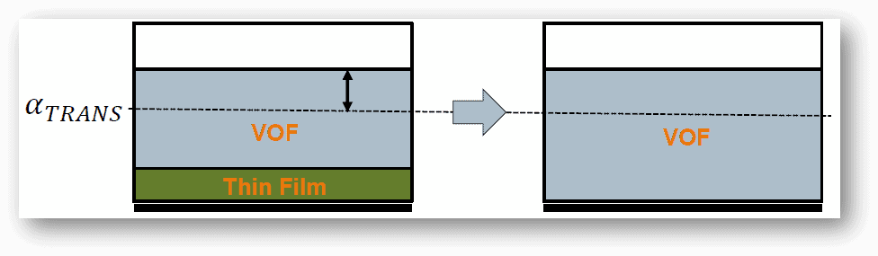
The fluid film model falls within the Eulerian framework and uses boundary layer approximations to predict the dynamic characteristic behaviour of wall films. The fluid film model is not a 2D-model type, but it is simulated on a thin shell of a solid wall. This wall can very well be a 3D-structure. However, the fluid film model assumes a velocity and temperature profile along the depth of the film and is not explicitly simulated. The fluid film model is often a good approximation of thinly formed fluids on solid structures that does not require full resolution through thin phase-structures. It can favourably be combined with VOF to allow for transition between fluid film and VOF at a user defined volume fraction.
DEM
The Discrete Element Model (DEM) is an extension of the Lagrangian multiphase model (LMP), that allows for more detailed simulation of individual particles. Instead of simulating parcels representing a cluster of particles, the DEM method will look at interactions between particles and interactions with particles and other boundaries. There are several particle models that can be simulated in Simcenter STAR-CCM+, where predefined shape models can be selected. You can also define your own arbitrary shape from 3D-CAD. You can include bonding between particles, simulated like emulating straws of grass or sheets of ice. Typical applications include simulation where inter particle interactions is of interest, like pills, capsules, or food particles. Note that this is an expensive way of performing simulations because each contact is modelled in detail and often with an increased number of particles comes an exponential increase in contacts and collisions.
EMP
The Eulerian multiphase model is the most complete, and therefore also the most advanced model when it comes to multiphase modelling. Conservation equations for mass, momentum and energy are treated for each phase separately, increasing the number of equations solved. Phases interact based on the contact area between the phases, making the length scales of your phases important, whether they are represented by dispersed or stratified flows. Running pure EMP simulations are in theory possible for all type of multiphase flows (except for dispersed solids), but there might be models that are better suited for the problem, since other models might capture the physics without being too computationally heavy.
MMP
The mixture multiphase model is an example of a simplified model type that originate in the EMP model. It can be used to model suspension-like multiphase flows. The assumption in this model is that the suspension is a homogenous single-phase system. This hold true when you can use weighted physical properties to represent a mixture of phases and solve momentum, mass, and energy for the mixture, but the phase fractions of the different phases are solved separately. You can also model slip velocity between phases.
DMP
The Dispersed multiphase model is a simplified model that focuses on a heavily dispersed phase in a continuous flow (<1% massfraction). The dispersed phase can be in any thermodynamic state, like gas, liquid or solid and in expected to follow the main flow. The coupling between phases is per default one-way, but a two-way coupling can be activated. The model works in a Eulerian manner but has aspects of the Langrangian framework in its modelling of the disperse phase. Typical applications are automotive soiling and aerospace icing. In the video below the DMP model is combined with fluid film to simulate water droplets as the dispersed phase on a car windshield.
VOF
Volume of fluid is a model is used to simulate two or more immiscible fluids, immiscible being the operative word. This model works best when each phase is represented by a large structure in the system. Meaning that the phase can be separated by a clear and sharp interface, typically free surface flow. What is of interest in VOF simulations are typically the movement of the interface between phases, making it a good option in the marine industry, but also for sloshing and wading simulations. The VOF method is in its core an interface tracking method, keeping track of the interphase between phases.
Multiphase course
At Volupe we have developed a multiphase course. This course can be tailored to fit your needs and to focus on the Multiphase models that you find relevant to your daily work. The course will go over the relevant theory for your applications and follow up with examples and workshops. Together we could look at what models to use to solve your engineering problem, and discussion will be encouraged because it is a big part of learning.
We hope this blog post has given you at least a short insight to the multiphase possibilities in Simcenter STAR-CCM+. Note that there are eons more to be written, not the least in the hybrid modelling capabilities provided by the software. If you have question on this or the multiphase course, do not hesitate to reach out to us at support@volupe.com.