How output is written in Simcenter Nastran differ between solution sequences. Starting from the ground up we have the SOL101 linear statics solution sequence offering quick and robust calculations for small strain, small displacement problems using linear materials. In SOL101 you simply ask for output, displacements, stress, contact results etc. and for each subcase defined you will have output. Since there is no load dependency, it is assumed that output is wanted for all defined load cases. Why would you otherwise have defined them? Moreover, results will be possible to scale due to the assumption of linearity. There is no point in extracting results at 10 %, 50 % or 75 % of the load. We can simply scale the final result to the corresponding load to see intermediate results.
In nonlinear solution sequences such as SOL401 and SOL402 the case is not as simple as for linear statics. Having the possibility to enable all kinds of nonlinearities: geometrical and material nonlinearities, as well as large strains and contacts, we are given a much more granular control of when output is to be given. For these nonlinear solution sequences, time is real in the sense that the solution will progress through time, even though dynamic effects can be neglected loads can still scale with time or can have a time dependent behaviour. Therefore, output can be extracted not only at subcase end times, but at select moments during these solutions. In todays blogpost we will take the time to review time step control options.
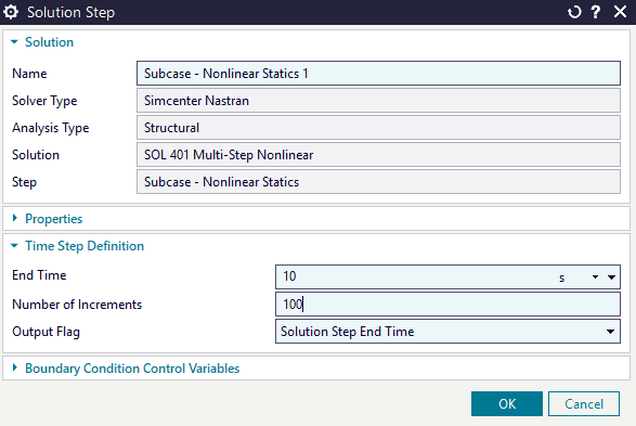
For both SOL401 and SOL402 the number of increments, output frequency and the time step length can be controlled for each subcase.
Right click the subcase → Edit → Time Step Definition group
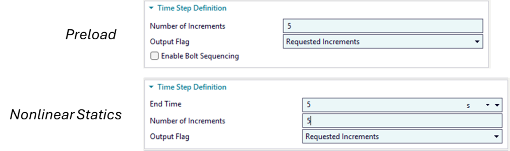
This will in the end modify a bulk data card TSTEP1 that will be controlling at which increments of the solution output is to be written:
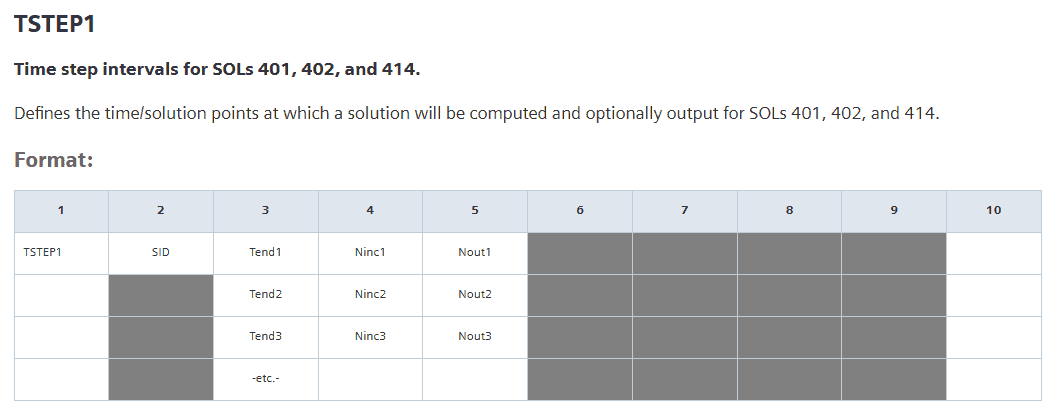
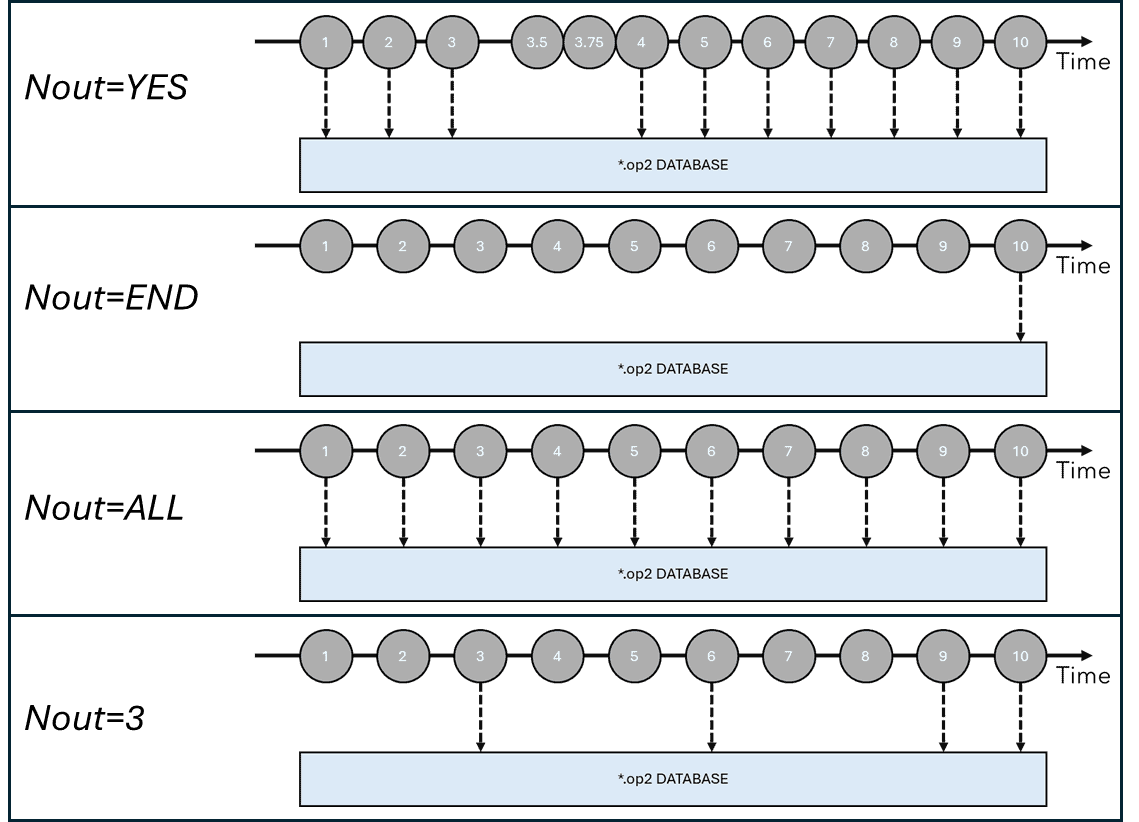
The structure of the TSTEP1 card is quite simple. It has a SID, just an ID which is referred to in the case control section of the input deck. Then comes the Tendi input (where the “i” is meant to be an index [1,2,3,4,…]) which defines the end time of the specific subcase in a sequence of potentially several subcases. How this specific subcase is to be split timewise into equal chunks is decided by Ninci input. Finally, the Nouti decides when output is to be written to the database with the values defined in the below table:
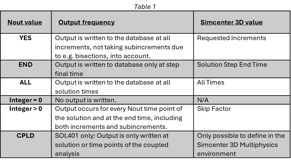
The output options can be summarized in the figure below where arrows indicate when output is written from an increment to the database:
If you wanted your structural solutions to run with fixed time steps this would be the end of it. However, using the bulk data entries NLCNTL, for SOL401 and NLCNTL2, for SOL402 you can activate and control adaptive time stepping based on the number of equilibrium iterations required for convergence. In SOL402 the adaptive time stepping is always active, but with the bulk data entry NLCNTL2 you can control the parameters of it. For SOL401 you will explicitly have to ask for adaptive time steps having AUTOTIM=ON and setting TSCEQ=ON.
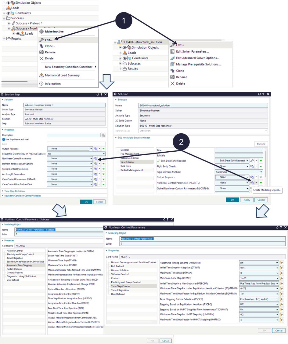
In Simcenter 3D you can activate and control these parameters either by modifying the solution:
right clicking your active solution → Edit → Case Control tab → create/modify Nonlinear Control Parameters
Or, by modifying a specific subcase:
right clicking a subcase → Edit → Case Control tab → create/modify Nonlinear Control Parameters
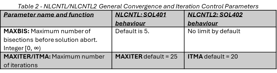
The parameters governing the adaptive time step behaviour in SOL401 and SOL402 are seen below in table 2 and table 3. Table 2 shows general parameters connected to convergence and iteration control. These are not directly coupled to the adaptive time stepping, but will affect it indirectly either by aborting the solution as for MAXBIS after sufficient amount of bisections, or as for the maximum number of iterations which will control the size of the next time step.

Adaptive time stepping using SOL401 and SOL402 will mean that the calculation of the next time step in the solution will become a function of how many iterations it took for the current time step to converge compared to how many iterations that the solver was allowed to make. For SOL402 one gets even more control when specifying the optimal number of iterations ITEREF which also will be taken into account when calculating the time step. Exactly how the time step is calculated is not disclosed by Siemens. In essence if a time step requires few iterations compared to the maximum to converge, the next time step will be increased with a factor proportional to EQMFMX. In opposite, if a calculation requires many iterations before it converges the next time step will be decreased with a factor proportional to EQMFMIN. Note that this cannot be used for constant time subcases, e.g. preload subcases. Then only the TSTEP1 parameters will be used.
Enabling adaptive time stepping will increase the complexity of the subcase setup since the subcases will take both the number of increments into account and at the same time they will have variable time step size between these increments. Effectively, using the previous example of having a subcase with an end time of 10 s, and having defined Ninc=10 increments will mean an initial time step of 10 s /10 = 1 s.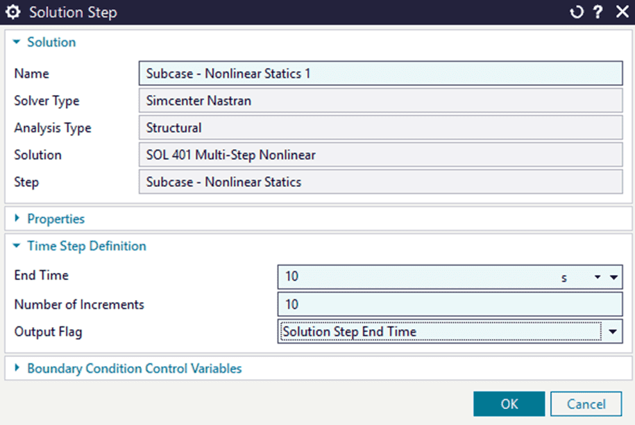
The adaptive time stepping will grant the possibility of subincrementing between the increments defined by the TSTEP1 card. E.g. between 1 s and 2 s the solver might take an additional step at 1.5 s if the number of iterations it took to solve the first 1 s time step was large. What needs to be remembered is that regardless of what the Nout parameter (Output Flag in SC3D) is set to, the Ninc (Number of Increments in SC3D) will still subdivide the solution into time increments. If the resulting time steps become sufficiently small, practically, the adaptive time stepping can be overruled.
Take the case above as an example where the timestep is 10 s long with 10 increments meaning that we will have 1 s long subcinrements decided by the TSTEP1 card. Let’s say the solver, with adaptive time steps enabled, wants to subincrement with time steps as low as 0.25 seconds. Potentially the solution will have 40 subincrements instead of the original 10. Keep in mind also that regardless of the increments, only the last increment for the solution step end time will be saved due to the Nout=END parameter, or as it is seen in SC3D Output Flag=Solution Step End Time.
Compare the last settings to these new ones were only the number of increments have been changed. Let’s pretend everything else is defined the same between these solutions. If the simulation we want to execute required timesteps as small as 0.25 s previously, the increments in this solution will be smaller than the timesteps what the solver calculated then. 10 s / 100 = 0.1 s increments. Thus, for a simulation such as this we would not notice the adaptive time stepping as the number of increments will force the solver to take time steps smaller than it would otherwise need. We should expect this solution to result in 100 increments, with no further subincrements added due to the adaptive time stepping.
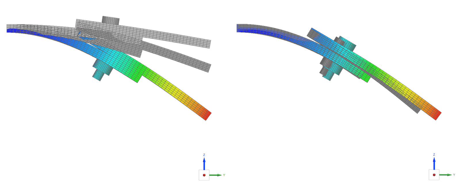
We need to remember that the Ninc parameter will enforce certain time points of the solution to be calculated. Another example is given below where the same simulation has been performed with differing settings for the Nout parameter while having adaptive time stepping enabled.
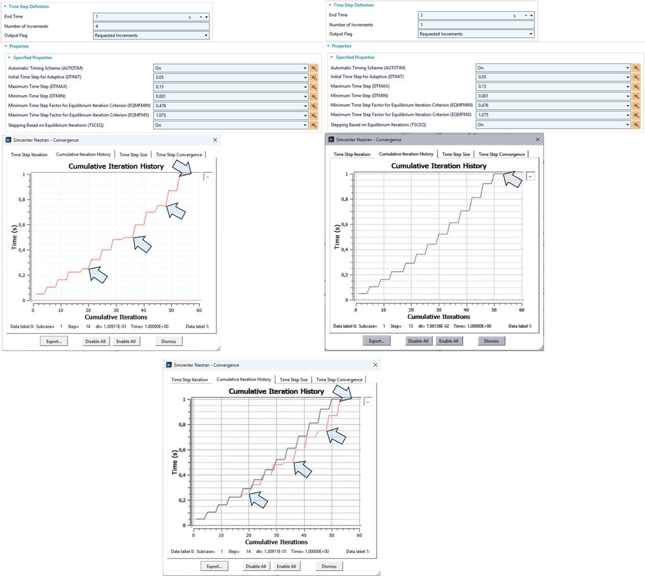
Here you can see to the upper left a simulation using 4 increments and adaptive time stepping resulting in several subincrements. Then there is the same simulation being solved to the upper right, but with only 1 increment and adaptive time stepping. The blue arrows indicate where in the time history that output is written to the database for each solution. Overlaying the Cumulative Iteration History plots of the two solutions, it becomes evident that the 4 increments of the left solution force the solver to sometimes take smaller steps than needed to “fit” into the defined increments. This can increase the solution time and if output is not strictly necessary from these time points one should refrain from enforcing increments in subcases.
Finally, how can one obtain results at specific time points while still utilising the adaptive time steps to their maximum? The answer is to skip asking the solver to create increments during subcases. If you wish to let the adaptive time step algorithm work with as much freedom as possible, you should stick to having one single increment for your subcases. Then, simply define your subcases with the End Time at which you require output and make sure you always output results at given time points by setting the Output Flag to Solution Step End Time to minimise writing to the database more than necessary -this will also decrease solver time.
Hopefully you learnt something new from this post and as always, you can send us questions at support@volupe.com if you are wondering about Simcenter 3D, Nastran or Femap.
Viktor Hultgren, M.Sc.
Contact: support@volupe.com
+46 704 21 06 61