A series of random load events are often described with the statistical based PSD theory, Power Spectra Density, or PSD in short.
The signals are quantified with the energy distribution across the frequencies.
A random signal is non-deterministic, which mean that the exact behaviour at any time in future cannot be predicted. However, the PSD theory applies to deterministic signals as well.
In this blog we will discuss the content behind the PSD and how it is often used in FE-simulations. Hopefully this will give insights of the basics in typical signal processing. Examples of PSD will be demonstrated on a deterministic sine signal.
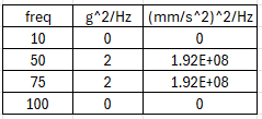
As a CAE engineer one often aims to load the structure with a random acceleration according to a frequency table:
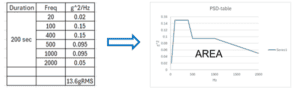
The energy of the signal is equal to area under the graph, and the given RMS is the square root of the area, so in this case the Energy=AREA=184g^2, giving 13.6g in RMS value.
If we now construct a “random” signal, with for example Simcenter Compose, and use some the information from the PSD table, a typical signal could be visualized accordingly.
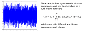
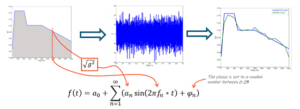
In this example we have constructed a time signal, based on the PSD table. Note, that the PSD table describing the average of several different random events. In this example we only have one random signal. However, it matches rather well when going back to a PSD description of the signal (green curve). General signal processing can as in this case be carried out with Simcenter Compose using predefined math functions, pwelch
Now, with this rather short introduction of PSD functions we now will look how it can be utilised in a FE solver, in this case Simcenter Optistruct and Simcenter Hypermesh as a pre-processor.
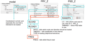
In order to solve the PSD spectrum in Simcenter Optistruct three load cases are needed
- modal analysis of the model, modes should typical be in the range of [0 to 1.5*(PSD freq max)]
- Frequence response analysis (often with a unit load which give the steady state response at the specified frequencies of interest) The unit load is often a unit acceleration in a specific direction, an = 1). The frequency loading is controlled via a FREQi card, for this simulation, FREQ1 has been used in Simcenter Optistruct.
Thera are different FREQi cards to used, some that utilise denser spacing close to the eigenmodes or linear spacing. - PSD load step, here you take the info from load case 2 and combine it with your PSD load curve.
A typical set-up could be that some kind of structure will be exposed to some random vibration, like this outdoor monitor exposed to some ground excitation, in this case vertical z-axis.
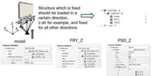
The three different load steps (or subcases) contain some different solver keywords, which are explained in image below. It is important that the shaker node, which was constrained in all d.o.f needs to be assigned a SPCD card in the direction of loading.
For simplicity a very simple model has been used as a demo model, just containing one flexible plastic part. The model is clamped in the left end with a RBE2 spider which then is excited in the z-direction, referencing a generic PSD table, here expressed in terms of (mm/s^2)^2.
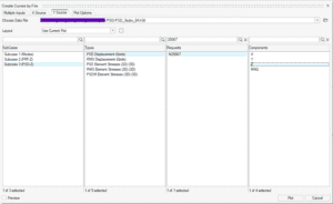
Result and postprocessing can now be done in Simcenter Hyperview and Simcenter Hypergraph. Given that the three subcases are performed the result file (.h3d) will contain information from all three. Detailed output can be requested in the pre-processing set-up in the subcase output option or in the global output. From the PSD-Z subcase the RMS displacement will be computed.
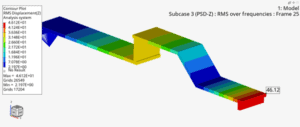
For the tip node in this case, the RMS displacement became 46.11 mm.
By plotting the PSD response over frequency for a specific node it will generates a curve which area under the curve corresponds to the total energy for this node. The RMS displacement will be the square root of this value, so by using the curve statistics icon in Simcenter Hypergraph one can inquire curve data, in this case the area value to 2126.9 giving the RMS displacement of 46.11 mm
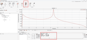
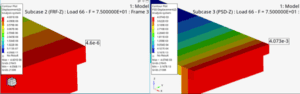
Closing the entire loop, from FRF to PSD to final RMS value these are the following steps that connect the results. For a given frequency, here 75Hz, plot the FRF displacement and the PSD displacement.
The PSD displacement will be the (FRF-disp)^2 times the PSD tabular value at this frequency. So, (4.6e-2)^2*1.925e8=0.004073, which is exactly the PSD displacement. Last step is to take the square root of the area under the curve for the same node to get the final RMS!
FRF -displacement PSD-Displacement
Hopefully you learnt something new regarding PSD and signals from this post and as always, you can send us questions at support@volupe.com if you are wondering about Simcenter Hypermesh, Simceneter Optistruct or Simcenter Hyperview.
Author

Johan Dahlberg
Contact: support@volupe.com