The liquids we use in our engineering applications typically always contain some trapped gas, generally air. This gas can be dissolved within the liquid, but if pressure is decreased the dissolved gas will be released back into its natural free state to form undissolved bubbles within the liquid. This process is called degasification. For the process of introducing more air, the term aeration is also commonly used.
As the liquid properties of a mixture can change significantly if gas is present in undissolved form, it is important to have methods to account for these phenomena. Both the impact of undissolved gases within a liquid, but also the process itself as well as rate of which gas dissolution and degasification take place.
In addition to degassing and dissolution, the liquid itself may vaporize to a gaseous state due to cavitation (pressure decrease) or evaporation/boiling (temperature increase). However, in this article we focus our attention on the process of adding or removing gases to and from liquid, and not the transition of a substance from liquid to gas itself.
To describe the principles of gas transport, three different options are implemented in Simcenter Amesim under fluid properties –> aeration/dissolution
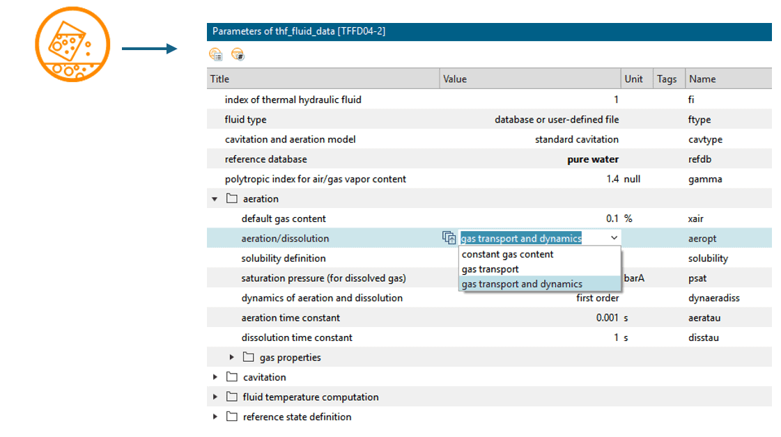
Constant Gas Content. The gas content is constant and the same everywhere in the system. This establishes that the mass fraction of gas remains constant in every volume present within the system. The amount of dissolved and undissolved gas may however vary between volumes. Thus, contrary to the total gas fraction, the fraction of dissolved and undissolved gas may vary from one volume to another. To determine the fractions, the local pressure in each volume is used together with Henry’s law and any dissolution or degasification taking place is considered to occur instantaneously.
While not a default variable in a volume when selecting the modelling approach “constant gas content”, the undissolved gas mass fraction can nevertheless be monitored by adding a “gas mass fraction sensor” next to a volume to sample its content. The fraction of gas present in the system is set by the parameter “default gas content”, and this is also the default aeration/dissolution model selected when adding a fluid properties component to the sketch.
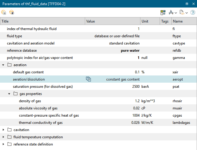
Along with the aeration/dissolution modelling approach, the properties of the trapped gas need to be defined.
Gas Transport. With this approach the total amount of gas is allowed to vary across the system, i.e. fractions may be different between individual volumes and the flow of gas between volumes is calculated. In addition to pressure and temperature, a new state variable is added for each volume to account for the total gas mass fraction, Xg. As will all state variables (#), an initial value must be set to initialize simulation. Here the default value is 0 [mg/kg] may be used, but users also have the option to use the built-in Gas mass fractions initialization assistant to set individual initialization values.
The evolution of Xg is computed at each timestep through the integration of dXg/dt, which is given through mass conservation in the considered volume element.
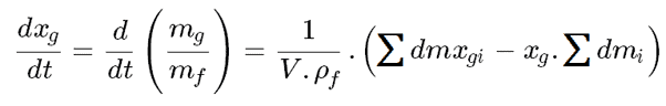
Where V is the volume, ρf is the density of the mixture of liquid, undissolved gas, dissolved gas, and vapor bubbles. dmi is the incoming mass flow rate and dmxgi is the incoming total gas mass flow rate.
For the Gas Transport approach the undissolved gas mass fraction is computed following Henry’s law, and again, dissolution and degasification phenomena are considered instantaneous processes.
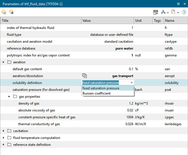
The Solubility Definition allows for the modelling of a fixed or a variable saturation pressure in the case of variable gas content. With the choice of Bunsen coefficient, the saturation pressure will depend on the volume element’s gas mass fraction.
The values for saturation pressure (or Bunsen coefficient) and of the default gas content have a large influence on the fluid properties and must be set carefully.
Gas Transport and Dynamics. Compared to the Gas Transport option, the dynamic processes of aeration and dissolution are considered. The undissolved amount of gas at equilibrium is still given by Henry’s law, but the current amount of undissolved gas, Xu, is computed from the application of mass conservation (similar to what was done for the total gas mass fraction, Xg). This approach is made possible by allowing both the total and the undissolved gas to flow between volume elements. This is contrary to the Gas Transport option where only transport of the total amount of gas is considered.
The time derivative of the total gas mass fraction is calculated following the same equation as given above for the Gas Transport approach. To add a similar equation for the quantity of undissolved gas, and allow it to vary from its value at equilibrium state (given by Henry’s law), an additional term is added to the end of the mass conservation equation.
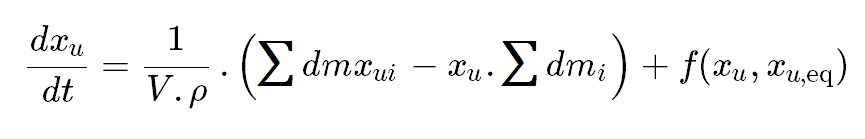
The function f(Xu, Xu_eq) determines the dynamic behavior of dissolution and degasification, and a selection for this expression can be set from the Dynamics of Aeration and Dissolution drop-down list.
The dynamic behavior can either be considered using a pre-configured first order lag or a user defined expression. The first order lag function is proportional to the undissolved fraction at equilibrium minus its current value, with an individual time constant (Tau) for the dissolution and degasification process.
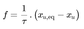
Usually, degasification is a faster phenomenon than dissolution and so the default degasification time constant is smaller than the default dissolution time constant.
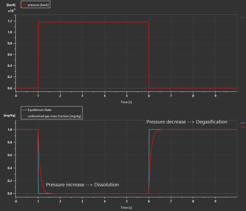
Below is an example showing the evolution of the undissolved gas mass fraction with its dynamics determined by the first order expression. In this simulation the fluid was subjected to harsh variations in pressure leading to both gas dissolution and air release.
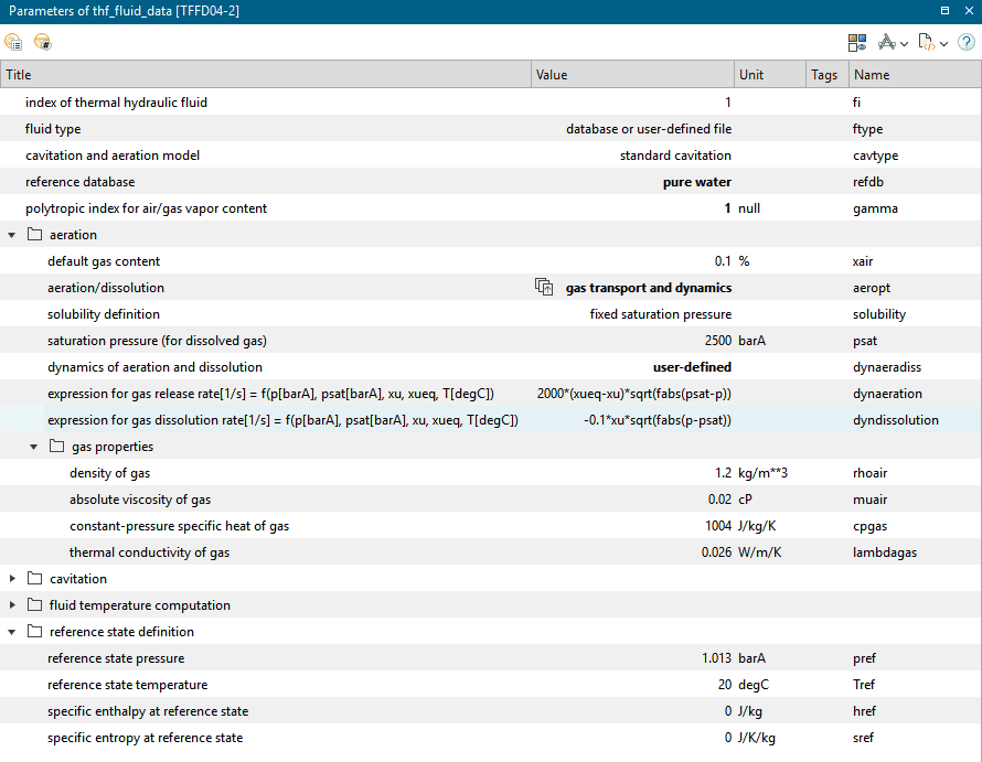
With the user-defined function, more complex dynamics may be studied compared to the first order lag. The proposed user-defined expression, shown when selecting this option, comes from a paper where the authors propose a set of simplified transport equations taking into account the effect of pressure on the air release/dissolve rate.
We hope you have found this article interesting. If you have any questions or comments, please feel free to reach out to us at support@volupe.com.
Author
Fabian Hasselby, M.sc.