Accumulated Force Table is a built-in feature in Simcenter STAR-CCM+ that is commonly used within external aerodynamics to visualize how drag or lift forces develop in the streamwise direction along a body. In this article we will demonstrate how to utilize this feature to analyze force distribution also in the spanwise direction, e.g. along the wingspan of an aircraft. Moreover, we will outline a workaround to overcome some of the inherent flaws that come into play with the Accumulated Force Table for the spanwise implementation. To demonstrate the workflow, we will use an example with a single wind-turbine blade.
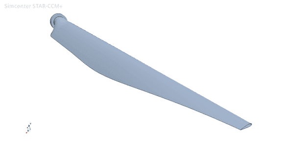
Spanwise lift force on a wind-turbine blade
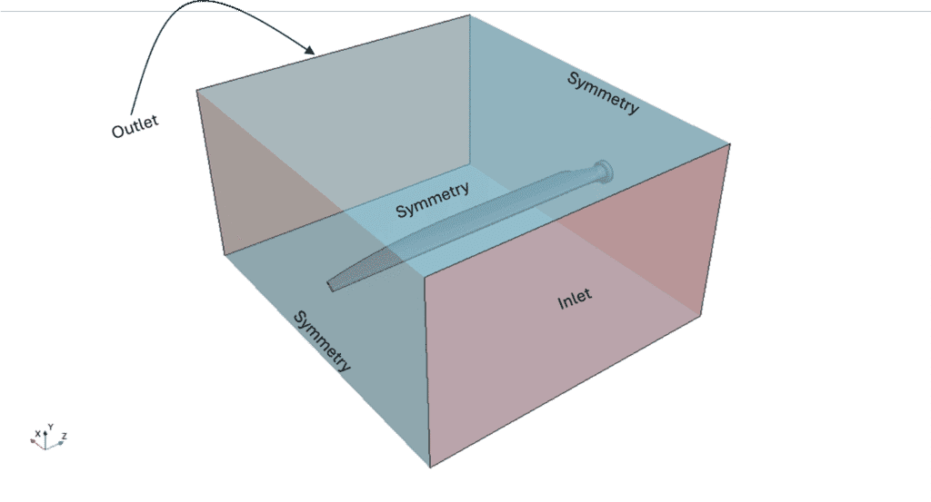
As mentioned above, the example case is a single wind-turbine blade, suspended in a box-shaped domain. The blade is subjected to an inlet flow of 10 m/s and the surrounding boundaries are modelled with symmetry condition to mimic a free-stream scenario.
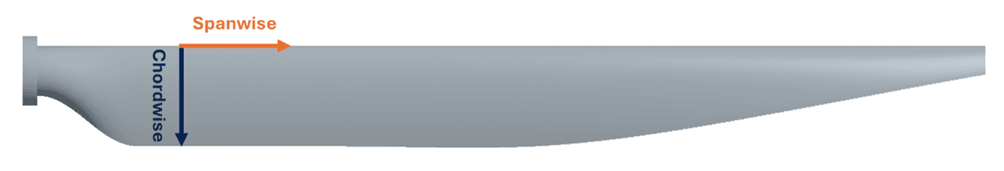
Now, let’s assume we are interested in knowing the spanwise lift force distribution on the blade (spanwise meaning in the direction from hub to tip, see schematic below).
As you may have guessed, we can utilize the pre-defined Accumulated Force Table to establish that. So, let’s go through that procedure.
We start by going to Tools -> Tables and create an Accumulated Force Table.
![]()
The Accumulated Force Table is basically a derivative from a histogram, where the ingoing parts are divided into “bins” (i.e. segments along a direction of choice), enabling presentation of data for individual segments. In this case, the ingoing parts are the upper and lower faces of the wind-turbine blade (see below).
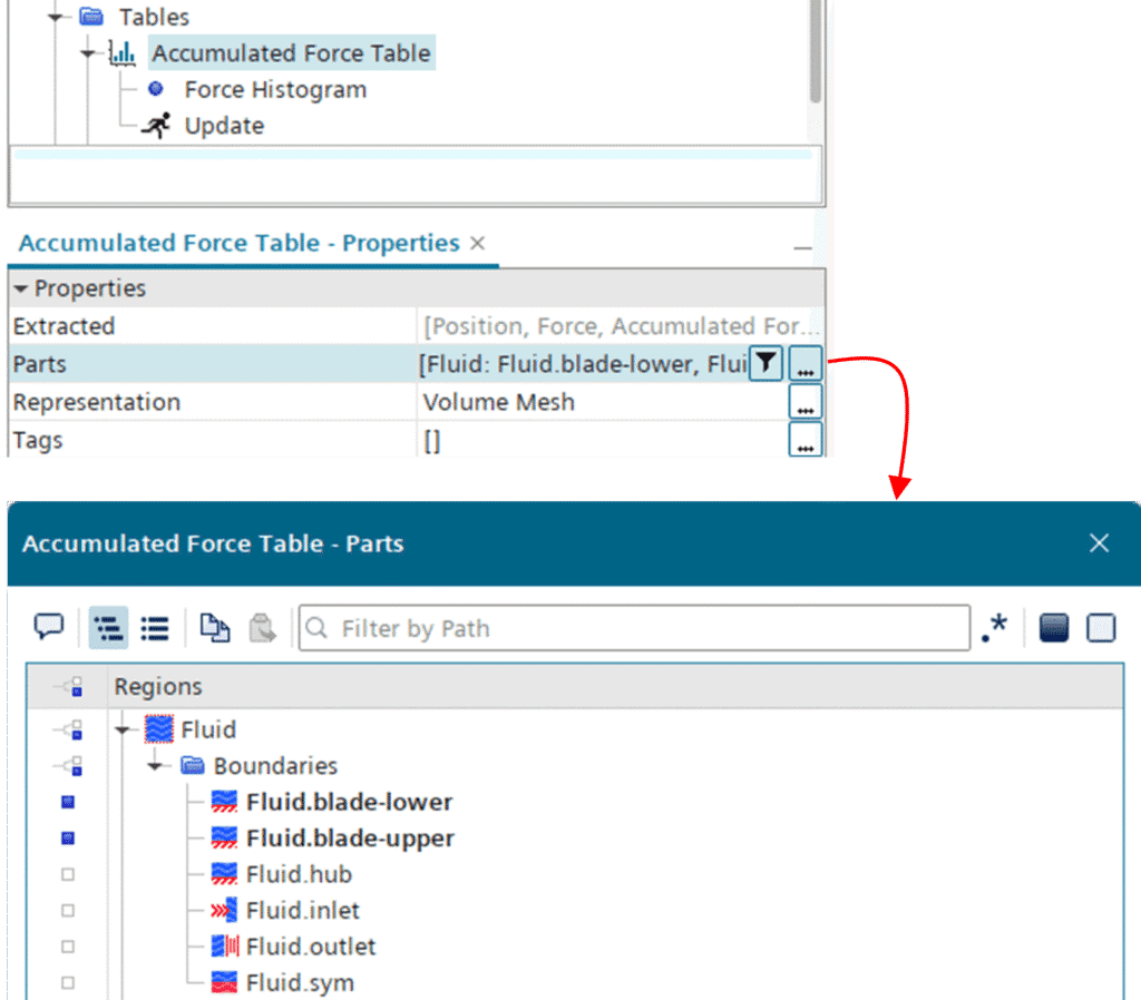
The underlying histogram requires input on number of bins (i.e. segments/divisions), the type of force, the direction of the force and the segmentation, any normalization constant (if you’re looking for a force coefficient) etc. In this example we decide to go for 20 bins sampled in the z-direction (i.e. hub to tip) and a force dependent on both pressure and shear in the y-direction (i.e. lift). You can see how all relevant properties are set up in the picture below.
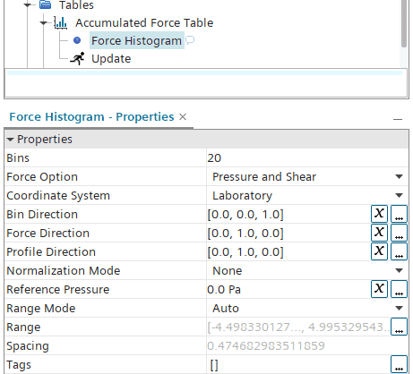
Once the properties are set up like this, we can extract the table data by right-clicking the Accumulated Force Table.
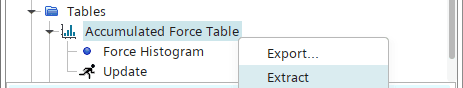
Now the data is ready to be used in an XY Plot.
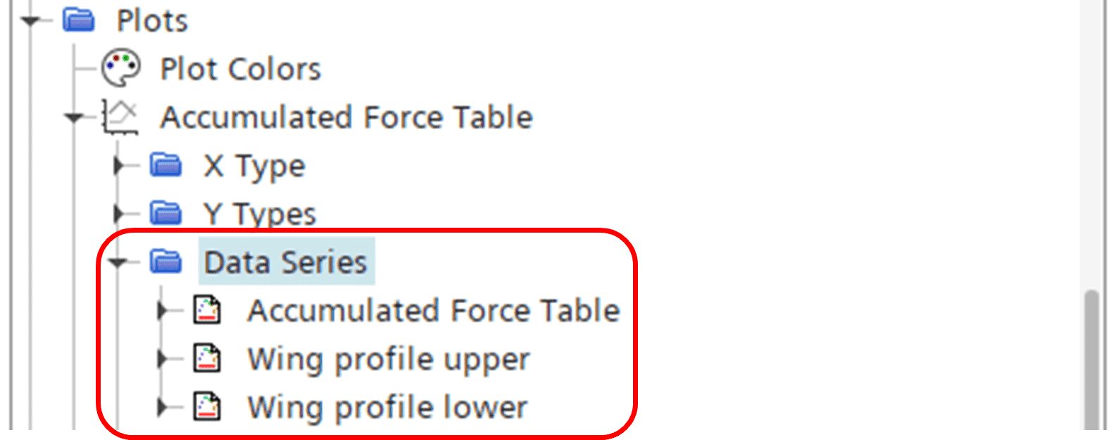
In the XY Plot, we can add the Accumulated Force Table to the “Data Series” folder (as shown below). You may note that there are two more entities under “Data Series” – Wing profile upper and Wing profile lower. This is because the Accumulated Force Table also provides a feature to divide the geometry contours into bins as well. This way you can plot also the geometry profile contours together with the force distribution, which can be quite useful for visualization purposes.
Although we are using a feature called Accumulated Force Table, the table itself contains also the local force for each segment, and not only the accumulated values. As depicted below, the table includes data on Accumulated Force, Force, Position, Profile Lower and Profile Upper. In this case we are interested in the local lift force contributions for each segment, so we choose Force as our input for the Y Column for the Accumulated Force Table entity. For the same reason, we use Position for the X Column, since we’re after the spanwise distribution.
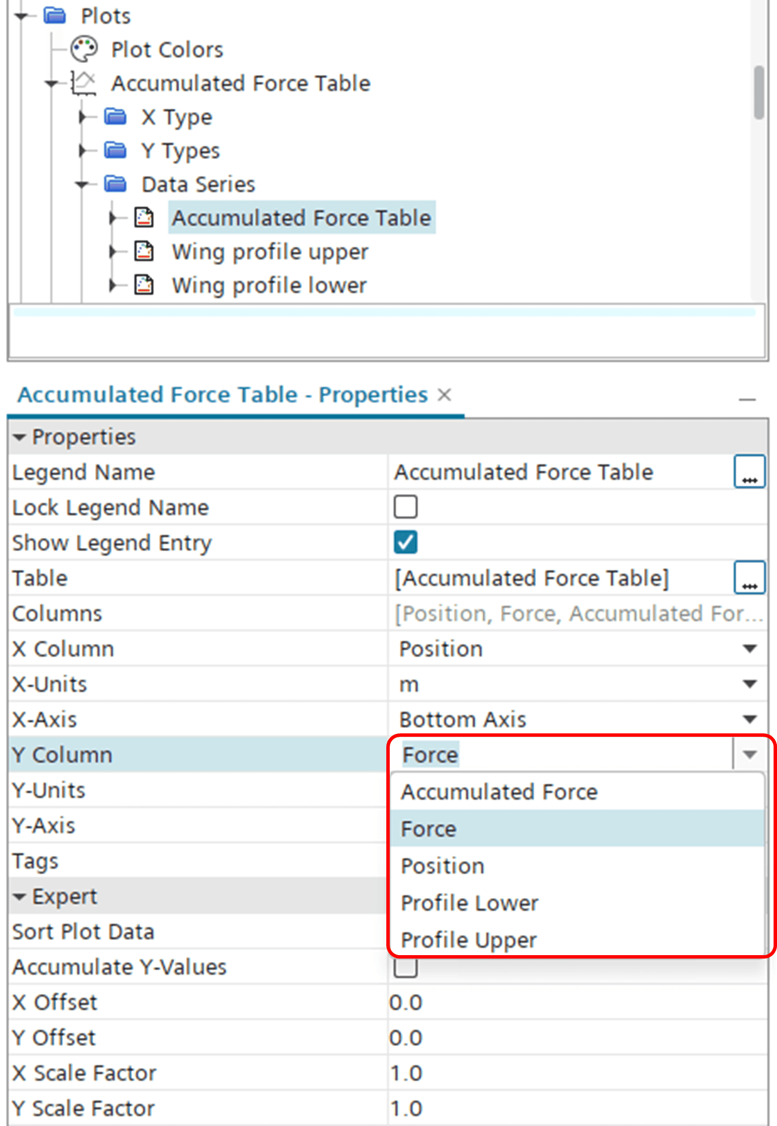
For the Wing profile upper and Wing profile lower data series, we select the Profile Upper and Profile Lower data, respectively. This will add the wind-turbine blade contours to the plot as well. In order to avoid a scaling mismatch between the Force and Profile data we put the profile Y Column data onto the right axis.
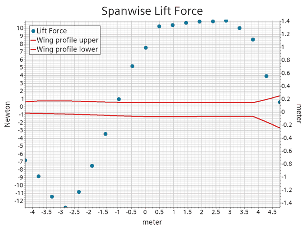
The final spanwise force distribution plot is shown below.
Increasing the resolution
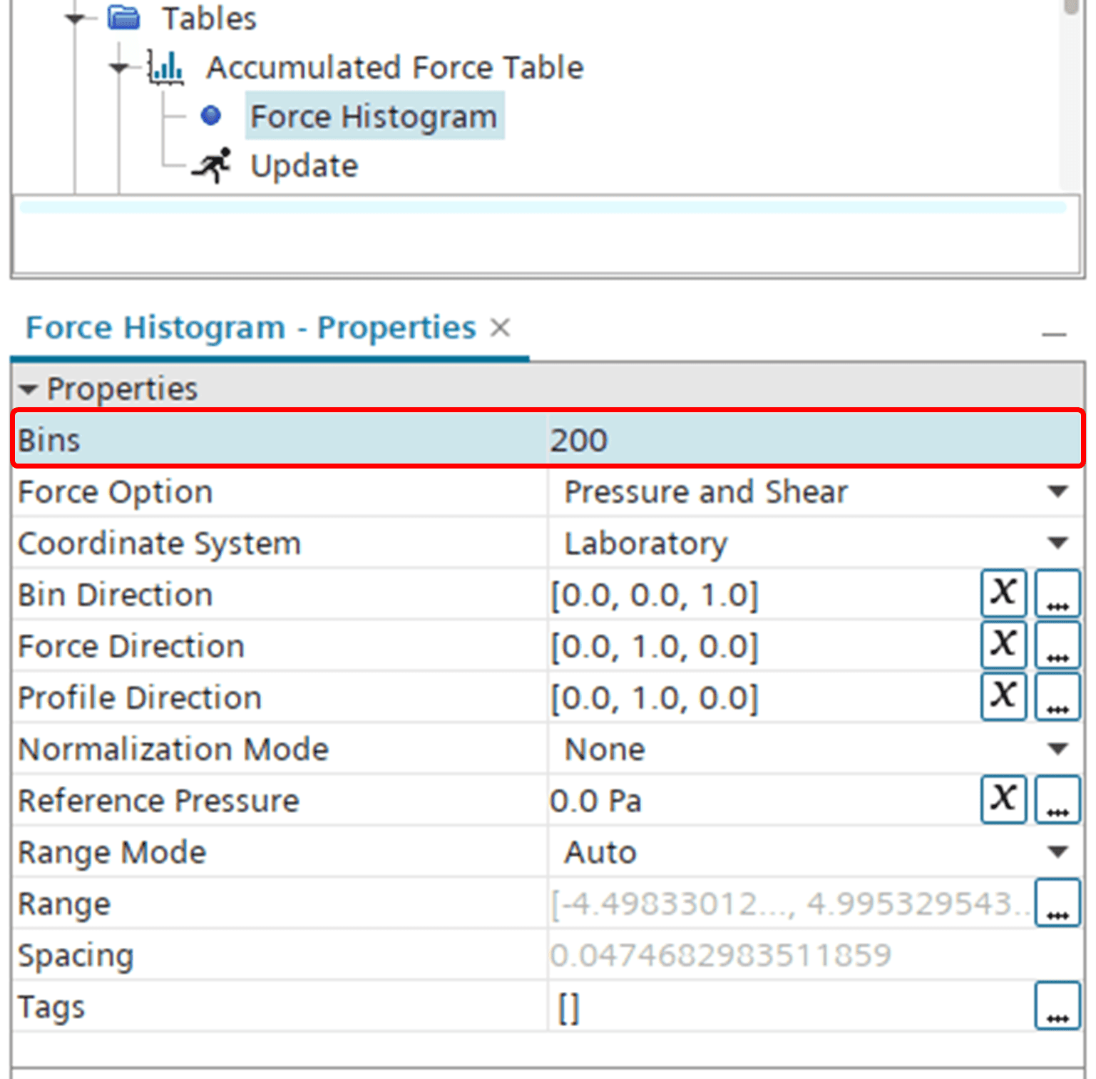
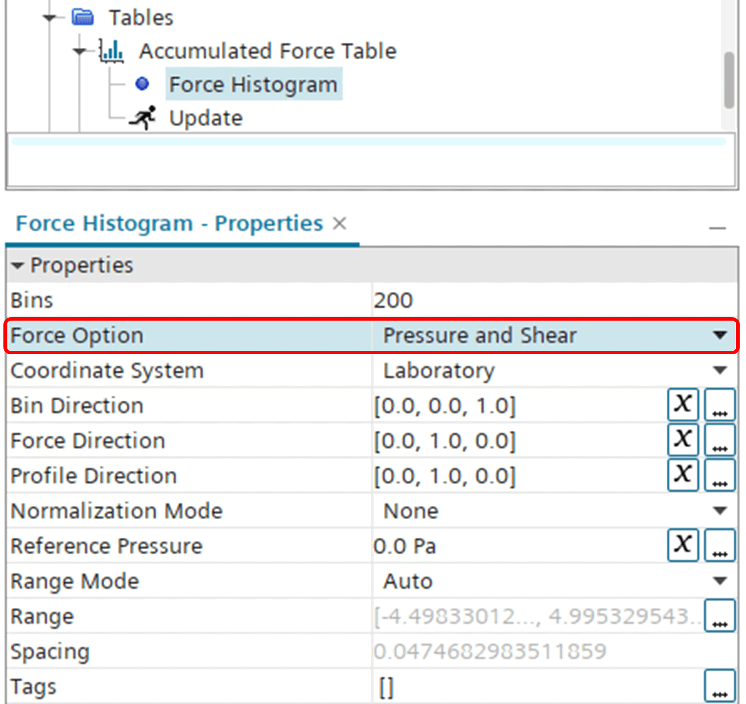
In some cases the plot achieved above is fully adequate, but what if we would like to increase the resolution of the distribution? Recalling that the division into segments of the ingoing part(s) is determined by the number of bins in the Accumulated Force Table, we move into the properties of the histogram and increase the amount from 20 to 200 (as depicted below).
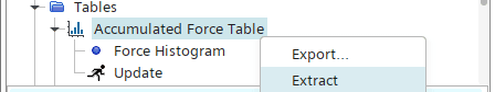
For the updated resolution to come into effect you need to re-extract the table values by right-clicking the Accumulated Force Table and selecting “Extract”.
Once this is done, the plot is updated with the increased resolution, looking like below.
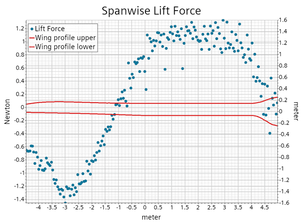
As you may note from the new plot, by increasing the resolution there is a lot of noise introduced in the distribution. The reason for this is due to the division of the unstructured mesh into bins. The division into bins only takes complete cells (or elements in this case) into account, meaning that there can be a slight imbalance in the number of elements in a segment belonging to the suction side and pressure side, respectively. This way there will be a slight biasing towards either suction side or pressure side for every second segment (or bin), making the output seem noisy. This effect becomes increasingly visible the more you increase the resolution (and effectively reduce the number of elements on each segment), since any biasing towards any of the sides becomes more influential the fewer elements the segment has. You can compare it to a statistical analysis, where any outlier or deviating response will have an increasing effect on the average for a smaller selection of data. If you increase the number of data points, the outlier becomes of less significance.
This type of noisy response is clearly undesirable when analyzing the spanwise lift distribution, since it gives uncertainties with regards to local effects. So, what can you do to improve the situation? In the following section we will outline a workaround to help overcome this noisy output.
Overcoming the noise
We just concluded that the noise is an effect from the decreasing number of elements on each segment of the wind-turbine blade. So, if we want to diminish the significance of the biasing towards suction or lift (i.e. decreasing the noise), we somehow need to increase the number of elements in each segment. One obvious solution would be to re-mesh the blade with an increased number of elements and simply re-run the case. But that is seldom a viable solution from a project perspective. So instead, we need to be creative.
In essence, we want to use the field data that we have, but on a (blade) mesh with finer resolution (i.e. more elements). The answer to make this happen is Data Mappers. Data Mappers gives us the possibility to re-use data from one mesh to another (e.g. for post-processing purposes). But this obviously also requires another mesh, so our first step is to generate a new surface mesh on the wind-turbine blade to use for post-processing the lift force.
Now, we need the new mesh to be decoupled from the original region and continuum, to not tamper with the solution we have. Also, we really only need a surface mesh for the post-processing, saving us some time not having to re-generate a complete volume mesh. To achieve this, we can make use of Shells. Since version 2402, there is a new geometry operation called Attached Shells Creator, allowing us to pipeline the creation of shells. Let’s add this operation to our pipeline. As the input part surfaces, we select the lower and upper sides of the wind-turbine blade (see below).
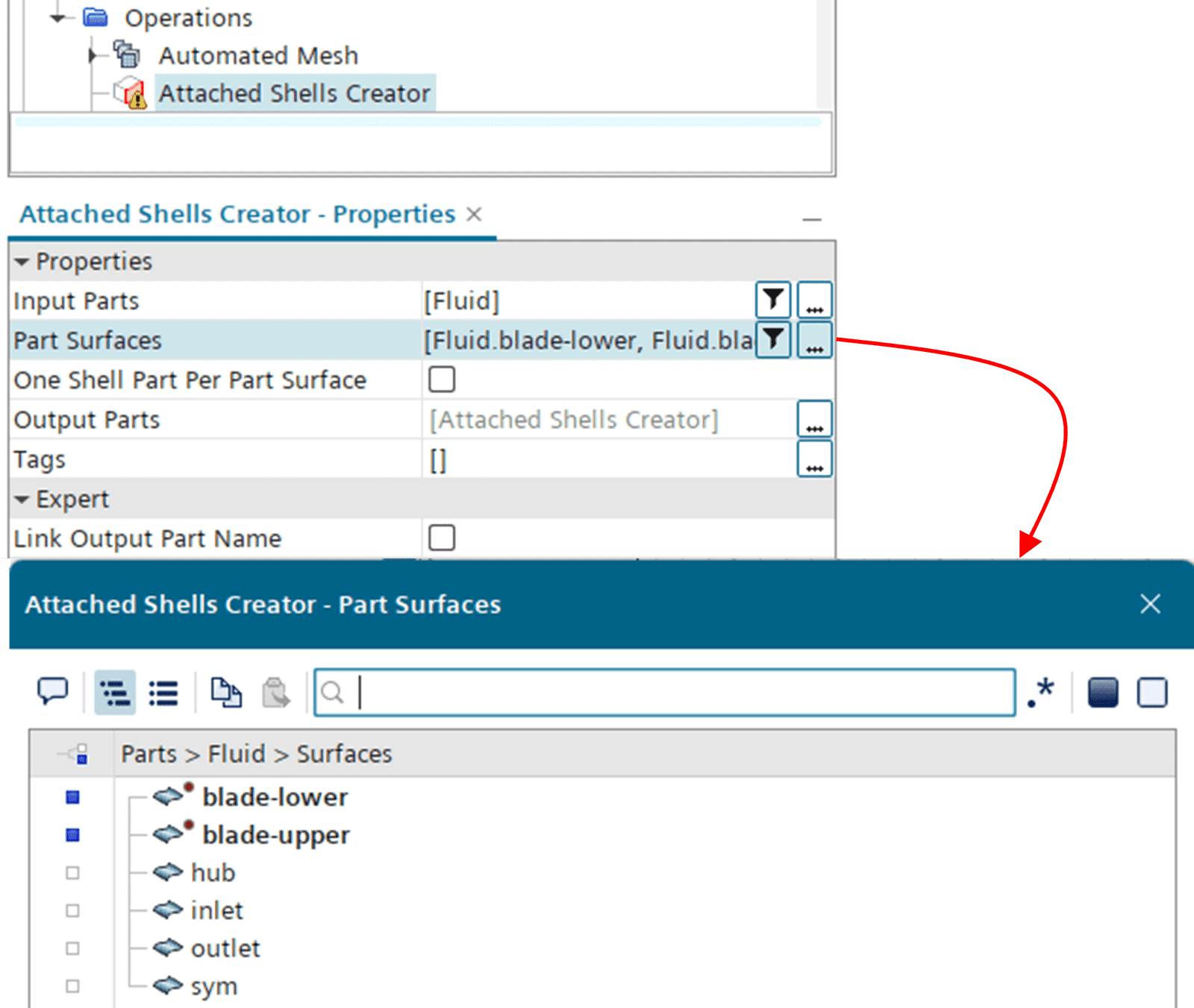
Creating the operation also generates an associated part in the Parts folder. This is the part that we will generate a new, refined mesh upon.
![]()
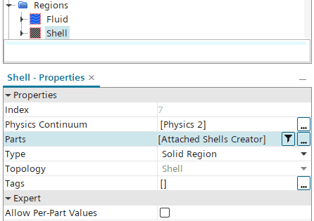
But, as always, before generating a mesh, we need to assign the new part to a region. In this case we let the Shells be associated with a solid continuum, since we are simply going to use it for post-processing.
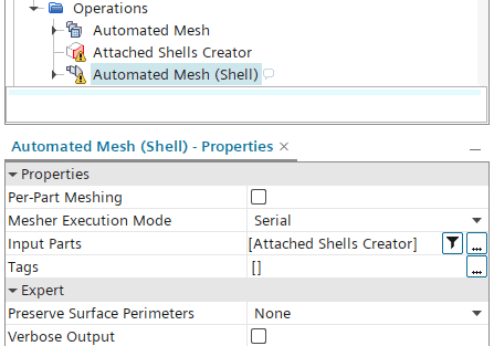
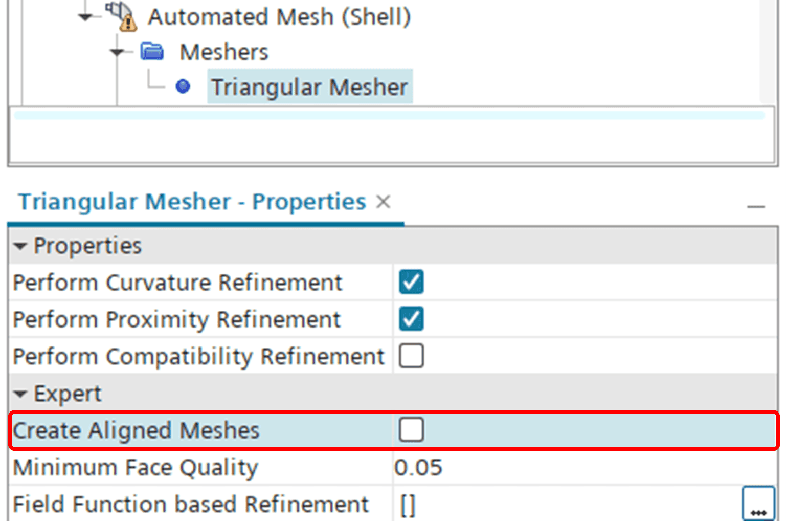
Next, we create a new mesh operation for the Shells. Since we are meshing a Shell part, and are only interested in a surface mesh, we add an Automated Mesh (Shell) operation to the pipeline. The input part to the operation is then the Attached Shells Creator part.
We select the Triangular Mesher, and in the Mesher properties we want to deselect the Expert setting “Create Aligned Meshes”. The reason for this is that we want to avoid clustering of cell faces to be included in the same bin. With an aligned mesh we could end up with entire element rows on either the suction or the pressure side, biased towards the same bin. This is exactly what we want to avoid, hence the deselection of this option.
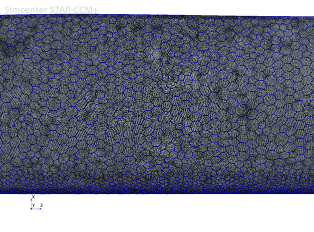
For the Default Controls, we lower the Base Size with 1/5 compared to the original volume mesh. Then we put the Target Surface Size and Minimum Surface Size to 20% of the Base Size (same number to attempt a somewhat equidistant mesh size on the blade). This will generate a substantially higher resolution on the Shell mesh compared to the Fluid volume mesh (which is what we want). Below is a picture comparing the original mesh (blue) with the refined Shell mesh (black) on parts of the blade.
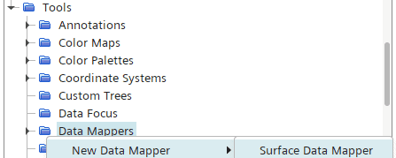
Next step is to map our data from the Fluid mesh to the Shell mesh. We go to Tools -> Data Mappers and right-click to create a Surface Data Mapper.
As Source Surfaces, we select the blade-upper and blade-lower faces, respectively. We also need to select what fields (or functions) we want to map. In this case we are interested in the aerodynamic lift force, so we need the pressure and the wall shear stress on the blade to evaluate that. Below is a picture of the Surface Data Mapper source properties.

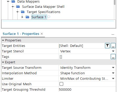
As our target, we simply select the Shell boundary (Shell: Default, see below). We keep the rest of the settings as default.
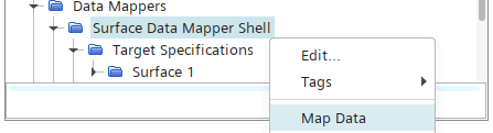
Once we are done with the Data Mapper setup, we can right-click the Surface Data Mapper and select Map Data.
Now we have successfully copied our pressure and wall shear stress fields from our original Fluid mesh onto our refined Shell mesh of the blade. Next up we want to use these fields and translate them into a lift force. In the case of an Accumulated Force Table, this is simply part of the input, recalling the input fields as highlighted below. The problem is that the Accumulated Force Table does not allow for mapped fields. So, once again, we need to be creative.
Recall that the Accumulated Force Table is in essence based on a histogram. Knowing this, we can create our own histogram, with the lift force based on the mapped field data as input. So, let’s begin with creating the lift force based on the mapped field data. We do this using a field function, let’s call it MappedLiftShell.
![]()
In the editor, we give the function the following definition, representing the lift force based on the mapped pressure and wall shear stress fields.
![]()
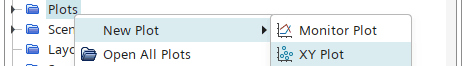
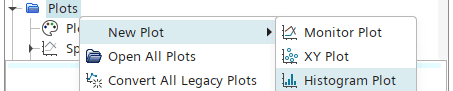
Now we are ready to set up a histogram plot for the mapped lift force. We go to Plots, right-click and select New Plot -> Histogram Plot.
The input part to the plot is set as the blade shells (i.e. Shell: Default, see below).
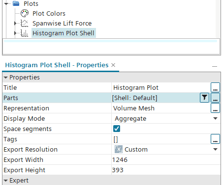
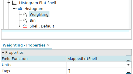
Moving on to the histogram properties, we set the number of bins to 200 (like the desired resolution from before). Moreover, we set the Weighting to Scalar Function, as we want to use the MappedLiftShell function that we defined earlier.
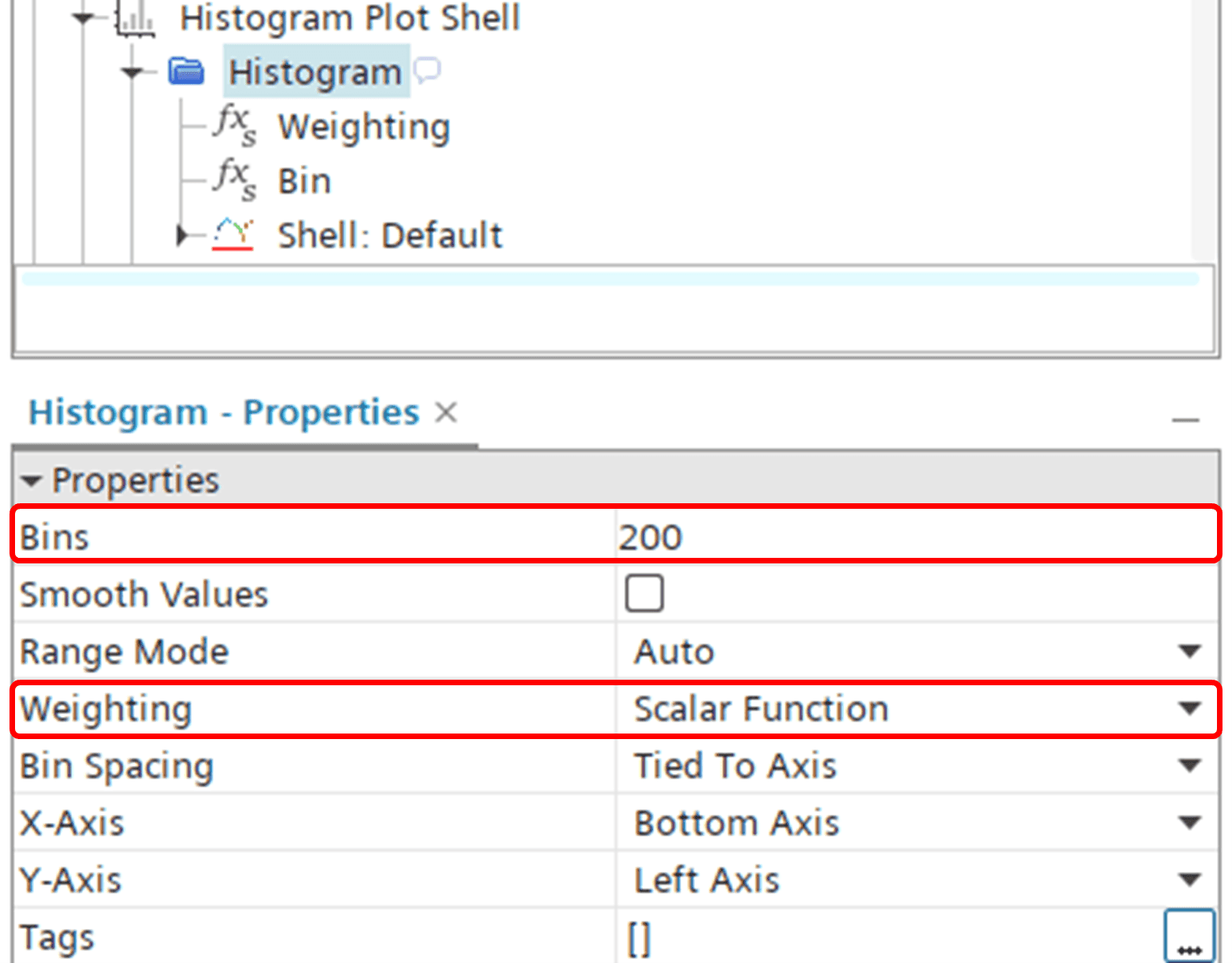
The field function itself is then selected inside the Weighting node.
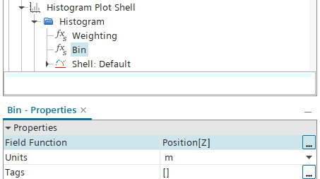
Similarly, we select the spanwise position (i.e. Position [Z]) inside the Bin node, since we want to visualize the spanwise lift force.
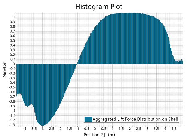
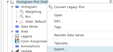
The resulting plot is a histogram like the one shown below. Now we want to plot the lift force distribution with point values rather than bars (as in the histogram) and compare with the data from the Accumulated Force Table. To do that, we need to export the histogram data to a file table, that we can use as input to the spanwise lift plot.
So, we start by right-clicking the histogram plot and selecting Export. Then we save the table data as MappedLiftShell.csv.
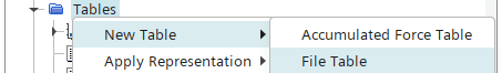
Then we move into the Tables folder and create a new File Table, selecting MappedLiftShell.csv as the input.
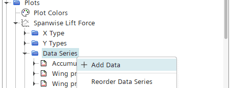
Lastly, we move into the Spanwise Lift Force plot, navigate into Data Series, right-click and select Add Data. Then we select the MappedLiftShell table as input.
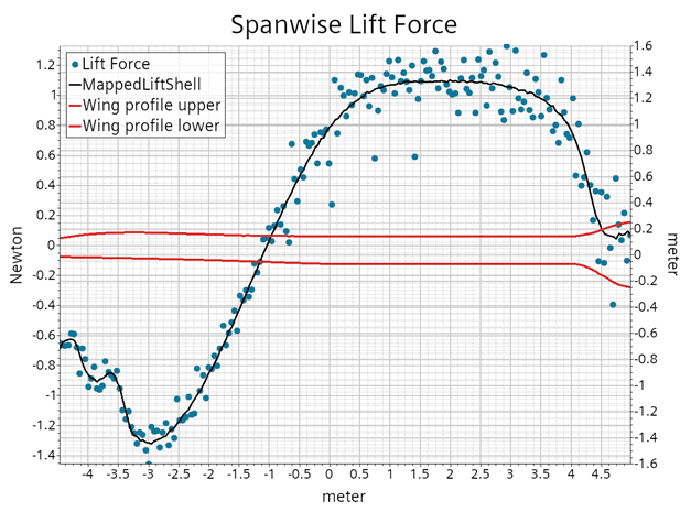
Now we are finally done with our workaround, and we can look at the comparison between the two approaches. In the picture below, you once again see the noisy output from the Accumulated Force Table (blue dots) alongside our refined output from our workaround with the Shell mesh (black line). As you can see, the workaround successfully gives us a more continuous look for the lift force distribution.
If you read all this way, I would like to thank you for showing interest. I hope you find this blog post useful. If you’re searching for more post-processing tips on e.g. aerodynamic performance, you can also read this post:
Turbomachinery Features – Single Section – Volupe
As always, feel free to reach out to us at support@volupe.com if you have any questions or comments.
Author

Johan Bernander, M.Sc.