In this week’s Volupe blogpost we will consider what is important when doing a CFD simulation using Simcenter STAR-CCM+, or any software for that matter. We will also investigate what happens when we decide to be pragmatic, when we allow ourselves to “cheat” a bit and adapt our simulation settings to the engineering question that we are working with.

General recommendations

In general, we learn that y+ value should be around 1, or at least that a y+=1 solution is somewhere the benchmark we should use. We learn that convective CFL number should be around 1 and timestep as small as possible to capture any transient effect that we have in the flow. For that matter, we also want our mesh to be as fine as possible, because we do not want to miss out on any geometrical features. For the mesh, we want a good mesh, with decent quality and transitions both between bulk and prism layers, as well as within the bulk, to land somewhere around 1-1.5 (my personal sweet spot is 1.2).

Some of these requirements put a big strain on the simulation, because a smaller mesh requires a smaller timestep to maintain the same convective courant number. A y+ value at 1 will almost always force us to use a larger number of layers to obtain the transition that is recommended. And while these recommendations are there for a reason, well established empirical recommendations, there are sometimes reasons to overlook some of them when we are solving certain problems. What is important to keep in mind is that it is not always necessary to resolve scales, both spatial and temporal, that are smaller than those of the question we are asking!

Convective courant number and CFL in Simcenter STAR-CCM+

In Simcenter STAR-CCM+ we have access to both convective Courant number as well as CFL number if we are using the implicit coupled solver. Those are not to be mixed up in the local terminology of Simcenter STAR-CCM+. While there is a general definition saying that CFL number and convective Courant number are the same thing, that is not how they are used in Simcenter STAR-CCM+. In Simcenter STAR-CCM+, the convective courant number is defined according to the picture below, this is in line with the general conception.

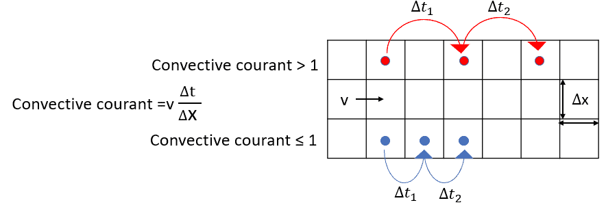
This is the traditional definition of not letting an imaginary point travel too far in a timestep, so that information is not lost, or the simulation becomes unstable or unphysical.

The CFL number in Simcenter STAR-CCM+ is a property for the Coupled implicit solver. The coupled solver conservation equations for mass, momentum and energy are solved simultaneously, advancing the solution through a pseudo timestep. This pseudo timestep is calculated from the CFL number specified. It is analogous to the under-relaxation factors used in the segregated solver. A smaller CFL number will give a smaller pseudo-timestep and the solution will require more iterations to converge but will hopefully stay more stable. Note that when using the coupled solver transiently it is extremely important to maintain a large enough number of inner iterations, since this is an under-relaxation factor. And with a low CFL number, i.e. a large under-relaxation of the solution you will, if not using enough inner iterations, push the correct solution in front of you inside the timestep. Making any time estimation being overestimated if this is not properly considered.

Solver type (implicit/explicit) and convective Courant number

Now we will consider the convective courant number in reference to the type of solver we are using. In Simcenter STAR-CCM+ we have the possibility of using Explicit and Implicit time-integration. In reality, it is only the coupled solver that can be used with explicit time integration, and that only when running the laminar or inviscid (something that only exists in the imagination) case. While this is important to remember from a practical point of view, it is also good to understand the difference between the two types of solvers. The Explicit solver only relies on what happened in the previous timestep, in the neighboring cell when deciding the current solution, while the implicit solver uses information from the previous time step as well as information from the current solution. Hopefully the picture below can provide a pictographic understanding of the methods.

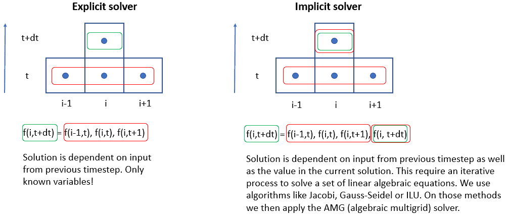
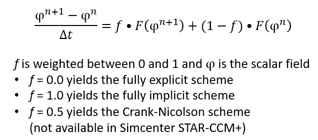
We can also consider this from a mathematical standpoint, then the description looks as follows. In Simcenter STAR-CCM+ you don’t provide the value you wish for f, but rather you select implicit or explicit time integration when selecting the Time-model.

This means that the Courant number becomes extremely important in an explicit solver, as that type of solver is limited by what happened in the last timestep. Any courant number above (or at least far above) 1 might lead to unphysical or unstable solutions. In Simcenter STAR-CCM+ you do not set the time-step size when using the Explicit solver, that is instead set by the Coupled solver and the size of that is related to the Courant number that you set. You can compare it to a completely unfiltered adaptive timestep, that has no chance of filtering out timescales that we think are too small. In reality the time step size is decided as the minimum value between the Courant number and the von Neumann stability conditions. Meaning at least that we will not go above the Courant number condition.

The implicit solver on the other hand has completely different requirements, there the CFL number for the coupled solver instead will set the conditions for the pseudo timestep in the Dual Time-Stepping methodology that is the Implicit solver. There you set the timestep, and with a large global timestep, you need to use either a large CFL (high under relaxation factor) or enough inner iterations to step through the pseudo timestep to a point where the solution is unaffected in the timestep. As with any simulation, find a solution that is time-step size independent. But twice!

This will allow for the Implicit solver to have a timestep that does not fulfill any requirements of a Convective courant number around 1. You can instead use whatever value suits your engineering questions without receiving an unstable solution. A larger time-step and with that a higher Convective courant number is possible as long as you stay within the scale that works in the same range as the dominant effect you have in your simulation. This can be hard to understand, so let us use an example to try to understand this.

Solving valve motion with DFBI and morphing with remeshing

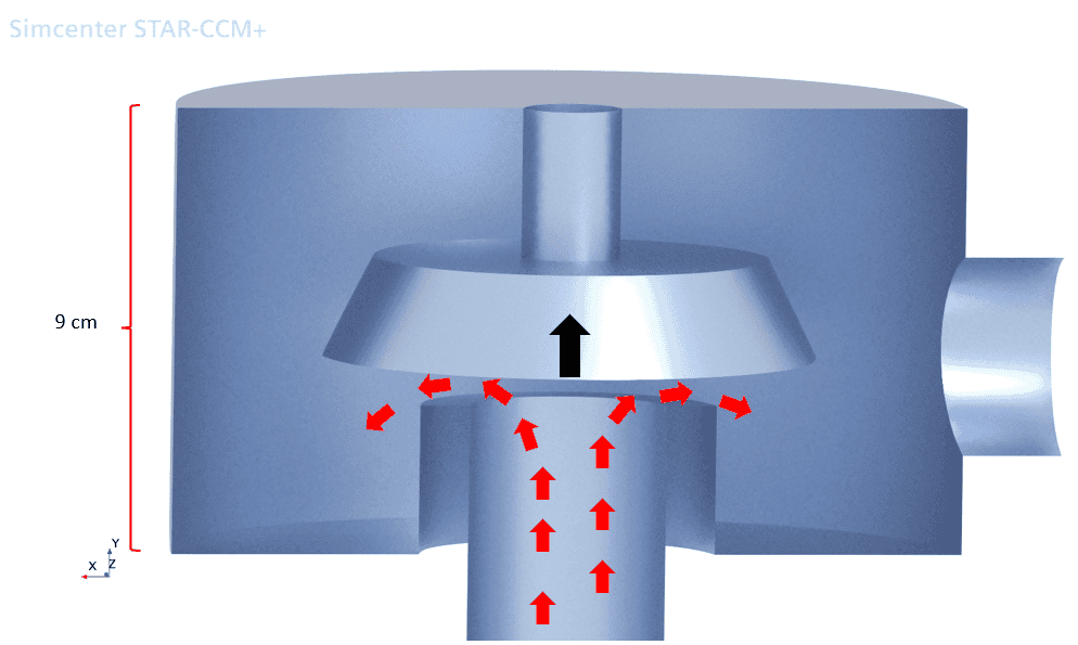
In a case where the opening of a valve from strong acceleration of a flow is applied, it is the body forces on the DFBI-body that dominate the result. If we wonder, how long does it take for my valve to open? We can with that question use a very pragmatic simulation setup to capture this phenomenon. I have prepared and run a case of a valve, defined as a DFBI body, attached to a spring (in the DFBI-setup). Below is a picture of the domain. It is simulated with symmetry. An increased pressure on the inlet is driving the flow and the spring up to its maximum degree of opening. The other physics applied here is DFBI morphing and remeshing of the domain at certain levels. From start to finish the valve is allowed to open 10 mm. The question we ask is; how long for the valve to open?

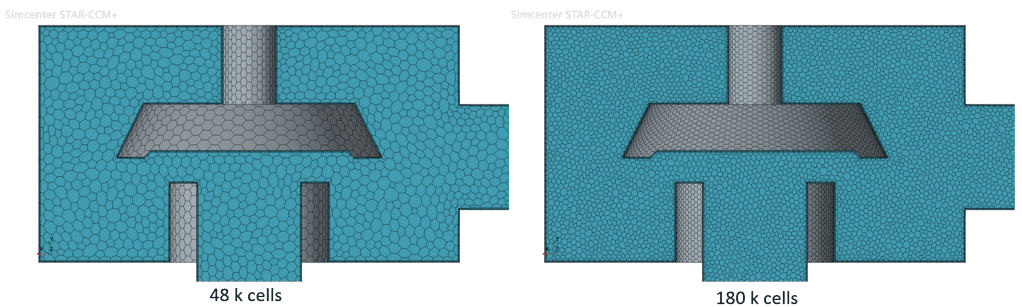
The pragmatic approach here is testing this with different timestep sizes and seeing what effect this has on the solution! I utilize a relatively coarse mesh on this, but test it also with a finer mesh. Bare in mind, that none of the meshes are extremely fine, but can give some sort of indication to whether or not we have a mesh independent solution. Below is a picture comparing the meshes, for the two different sizes selected. (The picture shows the mesh after full opening of the valve is achieved).

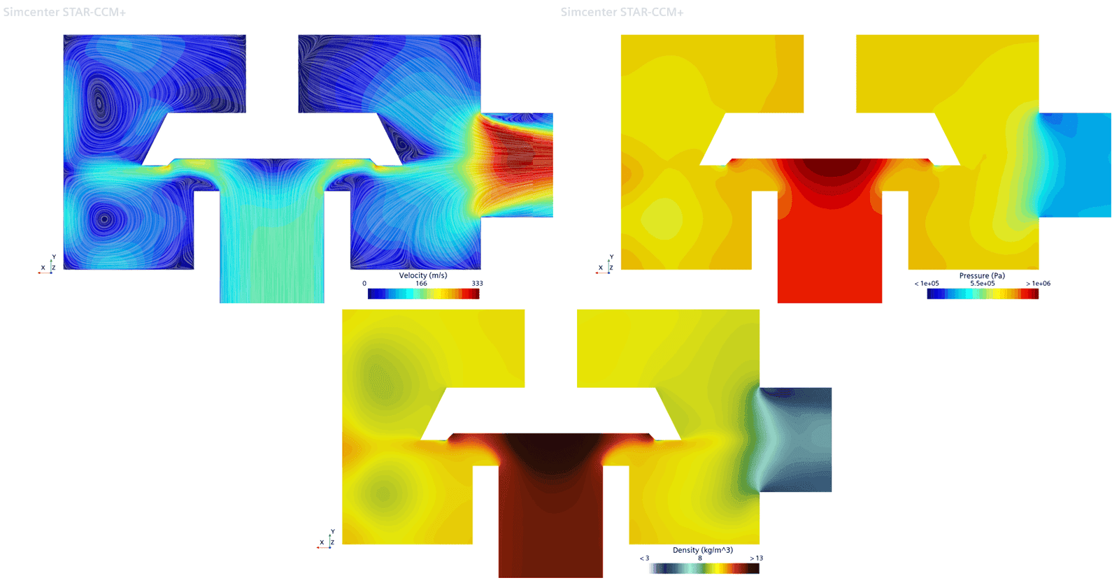
This sums up to six simulations, 2 meshes with 3 different timesteps. The timesteps selected were 1e-4, 1e-5 and 1e-6 seconds. A factor 100 in difference. The flow field was initialized with zero in velocity all over and the pressure on the inlet was instantaneously set to 10 bar. The picture below is to provide context into the results. These results come from the simulation with 180 k cells, and a timestep of 1e-6 s, the simulation that would be considered the one best resolved, both temporarily and spatially. This is at a stage where the valve is at its most open position, and the flow field has almost converged.

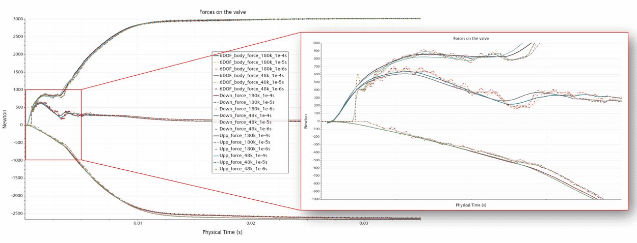
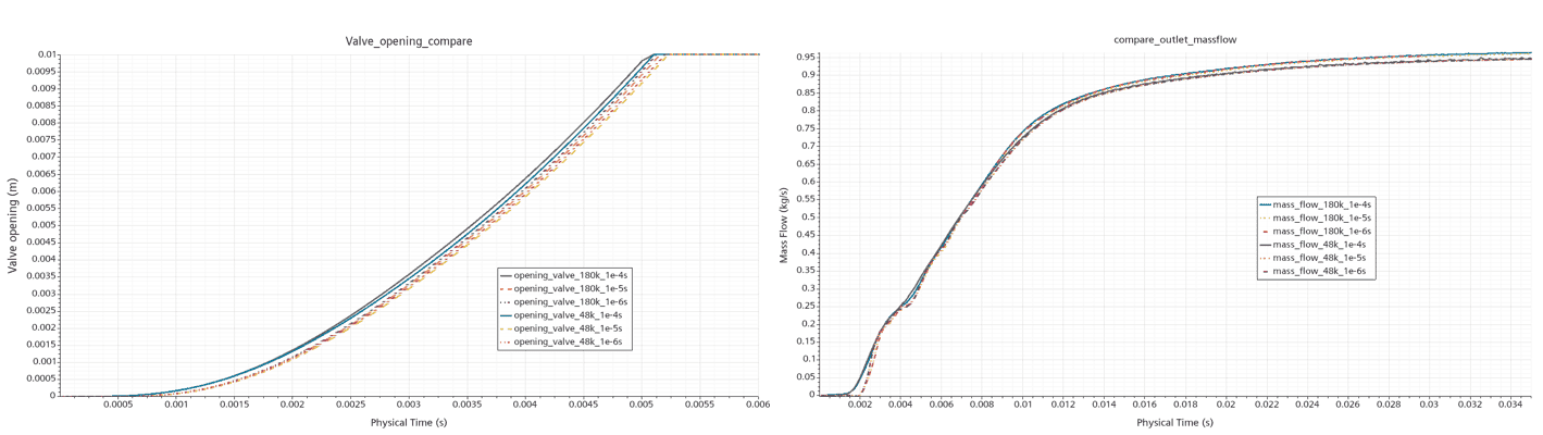
To evaluate this, the forces on the top and bottom part of the valve have been monitored, together with the DFBI force, on the DFBI-body. With this also the displacement of the valve and the mass flow on the outlet (both inlet and outlets are extruded in the simulation to provide distance to the area of interest). The top picture below shows the forces on the top, bottom, and combined body forces on the valve. Zooming in on the first few milliseconds is the most interesting part. On a small scale we can see that there are differences. The values for the smaller timescales are fluctuating, basically around that of the larger timestep. This means that there are transient effects that are resolved by the smallest timestep. However, looking at the opening time of the valve, that in all cases is evaluated to 5.1 (plus/minus 0.1) milliseconds, we see that any transient small-scale effect to the flow, and the forces, has small impact on the end result in terms of evaluating valve opening time for a certain pressure condition.

I hope this can help you understand that the highest level of resolution is not always necessary, but rather you can limit yourself to resolving the timescale interesting for the engineering question. And to understand what that is, comes with experience!

As usual, reach out to support@volupe.com with any questions.

Author

Robin Victor
+46731473121
support@volupe.com