Using Sliding Sample Window

There are several useful field function-monitors in Simcenter STAR-CCM+. The field function monitors available are:

Field co-variance — computes the co-variance of two field functions.
Field max — obtains the highest value of a field function for the selected part.
Field mean — obtains the average value of a field function for the selected part.
Field min — obtains the lowest value of a field function for the selected part.
Field sum — provides the total value of a field function for the selected part.
Field variance — computes the variance of a field function.

You can control these field functions using sliding sample window. The sliding sample window is the N most recent samples of data, (based on iteration or time-step depending on setup), during the simulation.

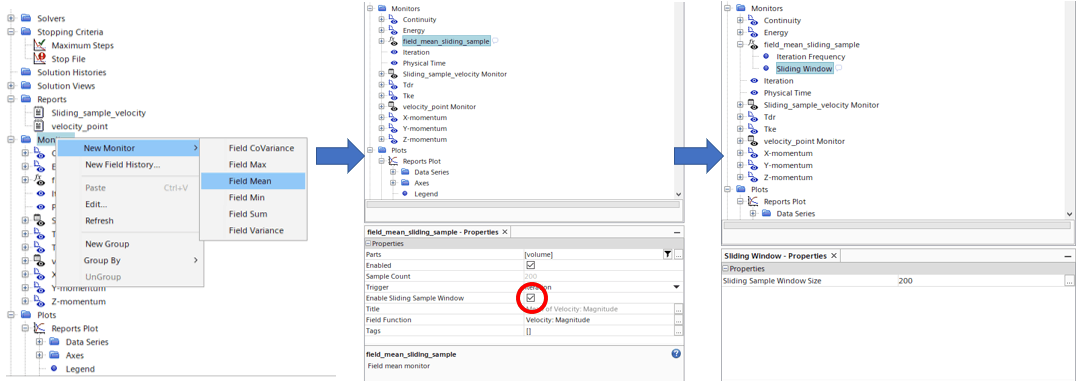
To evaluate this set of samples for a field function monitor, you need to activate the Enable Sliding Sample Window property of that monitor first.

This adds the Sliding Window node to the object tree under the parent field function monitor node. To specify the number of samples (the “window”), select this node and set the Sliding Sample Window Size property to the desired value in the properties window.

Example case

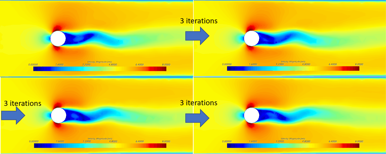
To show how this function can be useful imagine a simple case where a cylindrical pipe is crossing a slab and flow passes this cylinder, see the picture bellow.

In a case like this the velocity will not stabilise in the wake that is formed behind the obstacle. There will be transient effects in the flow. Something like the set of pictures below show.

However, if we still are interested in the average flow field over let us say 200 iterations, we can use the sliding sample window to evaluate the results. Assume that we evaluate the velocity in not only the entire field, but we also monitor the velocity in a specific point. See the picture below.

In our simulation we will monitor the velocity behind the obstacle, but we will also monitor the average velocity in the same point, over the last 200 iterations.

Create our monitor

To create the monitor, simply right click and create a new Field mean monitor (it can be any of the field function monitors). Under properties, tic in enable sliding sample window and set the number to 200.

We now have the monitor and we can create a field function pointing to that monitor and plot it in a scalar scene as we do with the velocity in each iteration. Create a new field function, name it properly and set the definition to point to the previously created monitor.

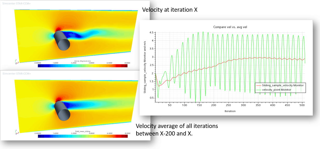
To evaluate our point value, simply create a report and select the previously created point and make sure you select the field function previously created. We can now plot the point velocity and the point velocity averaged over the last 200 iterations in the same graph.

After running this simple case for about 500 iterations we can compare the velocity field and the values associated with our point. The result can look something like below.

I hope this has been a useful tip. And as usual do not hesitate to contact me at robin.victor@volupe.com or at support@volupe.com if you have any questions in relation to this or anything else regarding Simcenter STAR-CCM+.

Example case

Create our monitor

Email opt-In Volupe