If you have ever had a simulation which was big, just a bit short of too many degrees of freedom (DOF), and you wished there was a way of simplifying it without affecting the results; Well, this blogpost could be for you. Using superelements in Simcenter 3D (SC3D) provides the chance for users to reduce the number of DOF in their models, freeing up RAM, as well as speeding up simulations without necessarily invoking a larger error in the analysis. How? Let’s have a look at how SC3D and Simcenter Nastran can solve this.
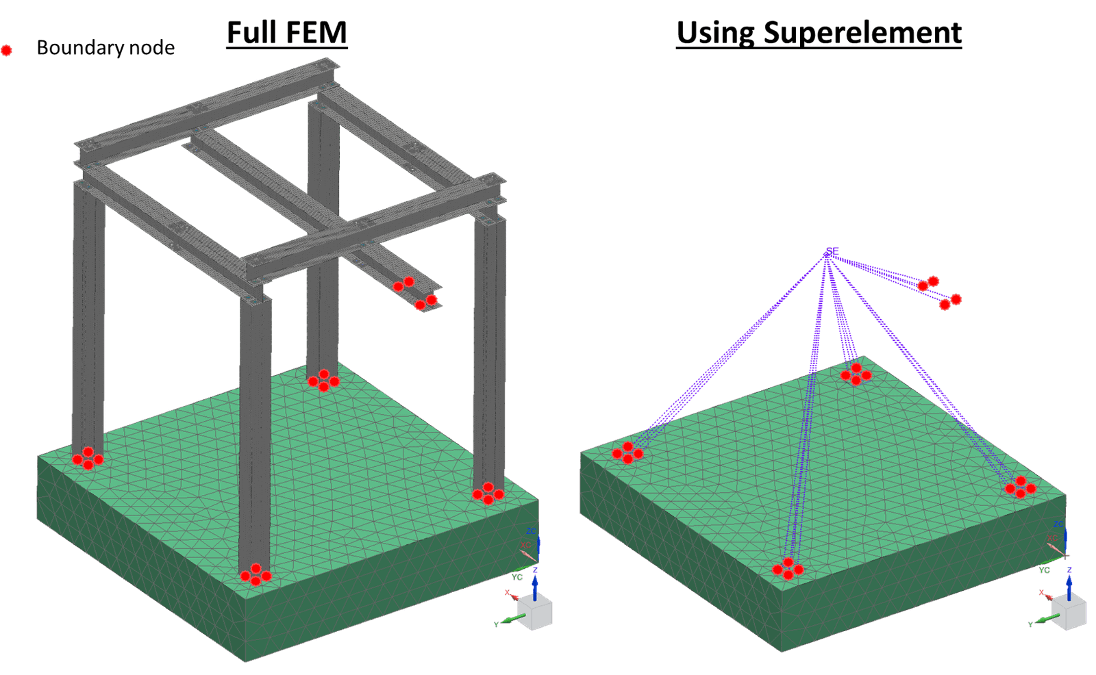
Starting off: what is a superelement? (Or SE, I will mix those two words as you tend to write “superelement” quite a few times in texts describing SE usage in your models.) An SE is a way of reducing the number of DOF in a finite element model from the original full set of nodes and their DOF, to only include the Boundary Nodes and their DOF. We then call the new “element” created in doing so a superelement and it will be combined with the Residual Model – which is the remainder of the model. Together these two form our System Solution.
When creating the SE, Nastran will create matrices describing the response in the full structure when the boundary degrees of freedom are displaced, as well as creating new stiffness, mass, and damping matrices for the SE. Thus, depending on how you output your SE you can also gain the advantage of not having to disclose any information of how the structure looks or functions besides where the Boundary Nodes are located and the mechanical properties connected to those nodes. Perfect if you want to send away your newest design to a partner company who needs it for an analysis, without giving away any restricted information.
You can create SEs both using static and dynamic reduction, in this post however, we will look at static reduction of the FEM only. As for the question of invoking errors in the analysis using SEs the SC Nastran Superelement User’s Guide explains it as follows:
“In static analysis the theory used in superelement processing is exact.”
Rarely has there been such a thing as a free lunch, and as you might have expected, the lunch is not entirely for free. Creating an SE will mean that another analysis must be solved. The final result can be quite cheap though, much depending on the size of the original FE model. The benefits increase the larger the original model was before reducing it, in combination with how many boundary DOF you choose to include. The fewer Boundary Nodes the better computational wise. It must be kept in mind that the above quote concerning the accuracy of the solution is with regards to static analysis. If we include the second part of the quote:
“In dynamics the reduction of the stiffness is exact, but approximations occur during the reduction of the mass and damping matrices.”
The errors compared to using a full FE model will be larger when performing dynamic analyses if a reduced model is used. To mitigate this there are ways of improving the approximations made in dynamic analysis using a different reduction technique named component mode synthesis. However, this goes beyond the scope of this blogpost.
Further down in this post we will see the impact of the approximations made to the mass and damping matrix when comparing results between a full FE model and one using External Superelements – meaning SE defined via input from an external file to the Nastran input deck.
So how can we use SEs in our SC3D analyses?
1 Preparing the Assembly
To use SEs in SC3D we need to start from an assembly FEM (.afm) and preferably have that associated to a part assembly. Then we will be able to replace FEM components of the assembly with their SE representations.
For those not familiar with assembly FEM files, they can be seen as a natural way of structuring an FE model in the same way as a part assembly in NX. If you want to place several instances of components in the same model, it makes more sense to input the same part file several times and position the parts, instead of creating several identical part files with different spatial placement of the part. As a note: assembly FEMs need not be associative. You can define them from several component .fem files not being related to any geometry.
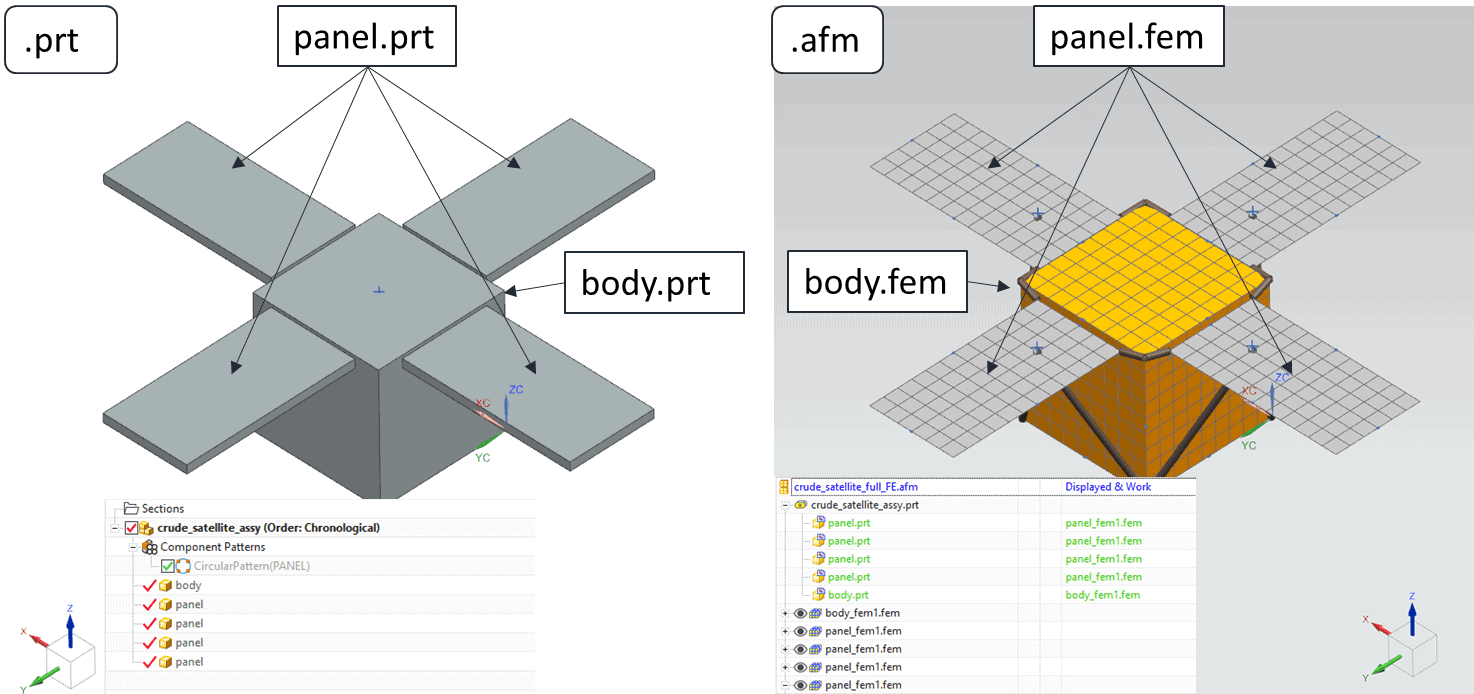
For this example, we already have an .afm file ready with a satellite consisting of 4 panels and a body seen below. On top of the bodies defined in the part files, linkages in the form of steel tube 1D elements have been defined on the assembly FEM level. Later we will see how these component FEM files can be changed to instead obtain their definition from external SEs.
On this FE model there are some simple point loads defined on the panels. Additionally, the bottom node, connected to the satellite body via RBE2 rigid couplings, prohibit any motion of the model by being constrained in all 6 DOFs.
2 Exchange Component FEMs for Superelements
Our goal is to exchange component FEMs in the .afm file for SE representations, then run the analysis and compare the results with our original FE model. To do this, first we need to create the SE representations from the component FEM files. Second, we need to create a new simulation and assembly FEM for comparison and in the new .afm input the SEs. Lastly, we need to redefine the simulation, rerun it, and then post the results. Let’s get to it!
2.1 Create a Condensation Simulation File for the Superelements
Before we can swap any existing FEM for a superelement we need to create one. So: How can an external superelement be created using SC3D? As stated, in this post we will only consider a superelement created via static condensation of the DOF (often this is referred to as a Guyan reduction), but the procedure is quite similar for a dynamically condensed one as well. To begin, we need a new simulation file which is associated only to the FEM we would like to reduce.
- Thus, we open the panel.fem used in the full FE assembly FEM and from this create a new simulation file. In this file we want the solution to be SOL 101 Superelement
- In contrast to a regular SOL101 static structural solution we do not have to define any constraints or loads in the solution to create a solution in static equilibrium. Instead, the Boundary Nodes must be specified. These are the only DOF which will be included with the external superelement into the system model. Thus, we need to define these at all interface nodes (connecting to other components) and nodes subject to boundary conditions.
- Either this can be done using the constraint: Fixed Boundary Degrees of Freedom
- Or you can define these nodes via the bulk data via editing the solution and thereafter creating a DOF Set.
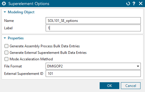
- To make sure we will obtain the correct output we will check the Superelement Options available under Edit Solution → Case Control. Here you can control the External Superelement ID written to the optional .asm and .pch files output if the Generate Assembly Process Bulk Data Entries or the Generate External Superelement Bulk Data Entries are enabled. Neither are required when we are creating the system solution inside of SC3D as the External Superelement ID and connection data will be assigned automatically by the program. It is also here that the output file format of the SE can be specified (being DMIGOP2 by default).
- Before solving we also need to make sure that the Output Requests in the reduction solution is a subset of the system solution output. In other words: If you want to look at stress or displacement of the SE later in your system solution, those outputs are required to be enabled already in the reduction stage, when the SE is created.
- Having set the Boundary Nodes, Output Requests and the Superelement Options for our reduction solution we can proceed and solve to obtain the <Solution name>_0.op2 file in which the superelement data is stored when the output file is set to DMIGOP2.

Note that for full pre- and postprocessing capability in SC3D the following formats are required to be output for the external superelements:
- *_0.op2 from a Simcenter Nastran SOL101 Superelement or SOL103 Superelement analysis.
- *.u18/*.sdb from a Simcenter Samcef Superelement Creation analysis or Simcenter Nastran SOL 414,103 Eigenvalues and Superelement Reduction in a rotor dynamics analysis.
In this example when we are solving a SOL 101 Superelement solution using the *_0.op2 format (DMIGOP2) will enable us to view the results of the SEs in the Post Processing Navigator. See below how the SE for the analysis is created:
2.2 Replace the Representation of the Component .fem Files in your Assembly to Superelements
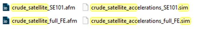
Having the external superelement ready to be included in an assembly FEM we will copy the existing assembly FEM and the corresponding .sim file to new *_SE101* files to be used with SEs.
By opening up the crude_satellite_accelerations_SE101.sim we can replace the associated FEM using the Replace FEM command and select the newly created crude_satellite_SE101.afm file. Having replaced the old assembly FEM, which relied on a model using component .fem files, we can activate the crude_satellite_SE101.afm and choose to Edit Representation of the panel.fem component FEMs in the .afm. When doing so we exchange their representation from conventional finite elements, stored in a .fem, to the external superelement we just created – panel_se_reduction-sol101_se_0.op2.
2.3 Run the Simulation
As we replaced the FEM in the .sim file, and we did not use Selection Recipes to define the point force loads, we are required to redefine them before solving. One thing to note is that the SE representations of the panels do not have any other nodes other than the Boundary Nodes selectable (as there are no other DOFs present from the SE in the system model).
After redefining the boundary conditions the solution is ready to be solved, requiring no extra input from our side:
2.4 Post the Simulation
Posting simulations where SEs have been included is straightforward: You just have to load results from the external SEs and then you can choose to plot the results from those SEs separately or choose to plot the residual structure with the SE results overlaid.
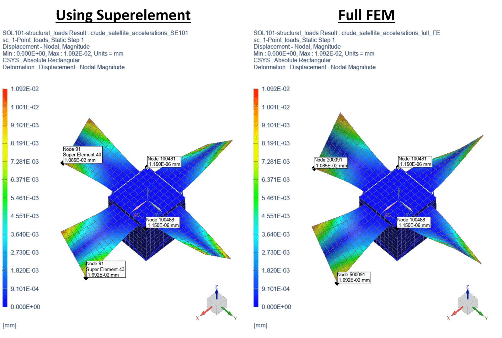
Moreover, as seen in the video and in the picture below, results between the static analysis correspond exactly with the results obtained using the corresponding FE mesh condensed into SE representations of the panels.
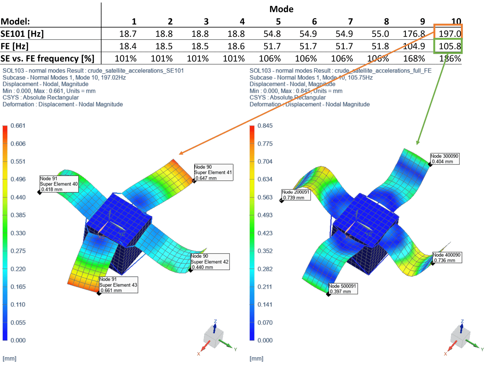
However, when looking at modal results from a normal modes analysis it becomes evident for higher modes that the correspondence between the system model and the full FE model breaks down. At mode 9 the eigenfrequency differs by a factor of 1.68.
3 Concluding Remarks
Using SEs in a System Solution created in SC3D is simple and can save you substantial amounts of time if large models are to be analysed. Moreover, it can provide ways of both dividing the model building work as well as protecting the design from being disclosed if sent to an external party.
Lastly, using External Superelements in SC3D is possible via tokens or package subscription. Then you can use SE modelling in all of these solutions (taken from the Pre/Post documentation):
- SOL 101 Linear Statics
- SOL 101 Superelement is not supported. You cannot condensate a new SE using SE in the same solution.
- SOL 103 Real Eigenvalues
- SOL 103 Superelement, SOL 103 Flexible Body, and SOL 103 Response Dynamics are not supported.
- SOL 105 Linear Buckling
- SOL 107 Direct Complex Eigenvalues
- SOL 108 Direct Frequency Response
- SOL 109 Direct Transient Response
- SOL 111 Modal Frequency Response
- SOL 112 Modal Transient Response
- SOL 402 Multi-Step Nonlinear Kinematics
For this post I used Simcenter 3D version 2412.6000. I hope it was of use to you. If you are having trouble using superelements in SC3D, contact us at support@volupe.com.
Viktor Hultgren, M.Sc.
Contact: support@volupe.com
+46 704 21 06 61