This year’s last Volupe blog post will be in a different format than usual. We will have a look at some simulations about badminton shuttles. I, Christoffer, have played badminton for as long as I can remember and when I studied at Chalmers University of Technology, I got the opportunity to combine my favorite sport with my engineering work.
At Chalmers they are doing both experimental testing and calculations for badminton shuttles, with the end goal to be able to design new plastic badminton shuttles that behave as organic feather shuttles. Chalmers and Volupe are now looking into how Simcenter STAR-CCM+ can help predict the behavior of badminton shuttles, and this blog post will be describing some of the focus areas that we have covered so far – but luckily there are many topics still to investigate so we can continue to work together within this exciting area of sports combined with physics.
Additionally, the idea behind the blog post is also to explain and cover technical aspects that will be of use in other applications. I believe this is a good case study to demonstrate several Simcenter STAR-CCM+ features and how to combine them, and hope that it will be of great use even if you are simulating other things than badminton shuttles.
Introduction
When simulating real case simulations in detail there are always many topics and details to consider. For badminton shuttles the trajectory of different strikes would be very interesting to define, to make sure that the flight will be accurately predicted and validated towards experiments. To get an accurate simulation of a strike, physical aspects like forces from the racquet, moment of inertia for the shuttle, Magnus effect when the shuttle starts to rotate, compression of the feathers etc should be taken into account. But since the numerical strategy must be validated first, giving that discretization and turbulence models, etc. has to be validated to capture the physics in an accurate way, some limitations have to be done in the first simulations. Therefore, we have started to look at mesh resolution, and how good the overset mesh methodology works for a simplified simulation and limit the scope to only look at a serve strike (shuttle going forward pointing upwards, with medium power, to then fall down). No FSI, Fluid-solid-interaction, for example the compression of the feathers is considered yet. But three different geometries are used to predict how folding of the feathers can impact the flight (in badminton, you fold the top of the feathers to create some extra drag which lowers the speed of the shuttle if there are too fast conditions).
Table of Contents
- Geometry
- Base geometry
- Folded shuttles
- Mesh strategy
- Moving meshes
- Overset mesh
- Comparison with other strategies for moving meshes
- Refinements
- Default controls
- Wake refinements
- Moving meshes
- DFBI
- Coordinate system
- Moment of inertia
- Force
- Solver settings
- Time step
- Turbulence models
- K-epsilon
- DES
- Simulation results
- Trajectories and flow path
- Comparisons with different solver settings
- DES
- New moment of inertia
- Post-processing
- Conclusions
- Future work
- FSI
- Turing of shuttle (tumbling)
- Plastic shuttles
Geometry
There are many brands when it comes to badminton shuttles, but the ones used for professional competitions look fairly similar.
Folded shuttles
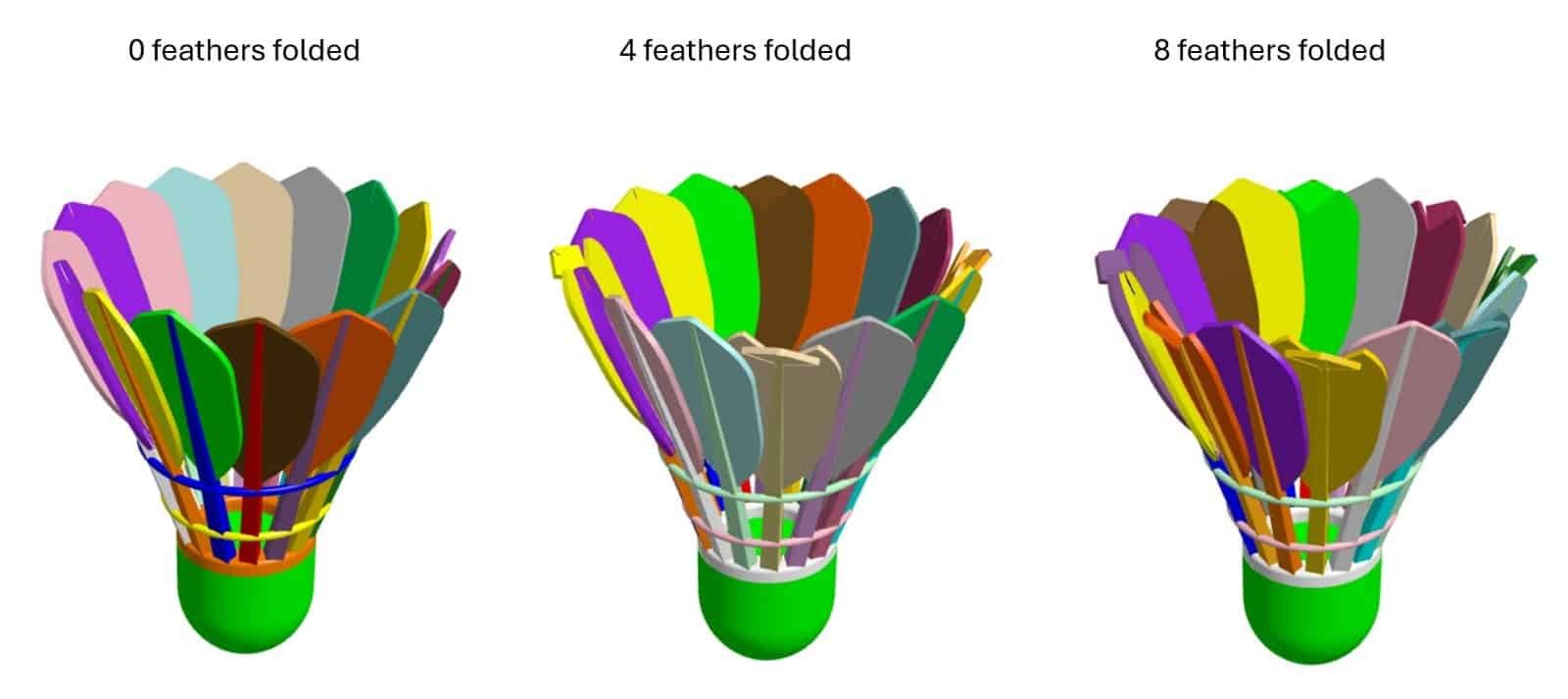
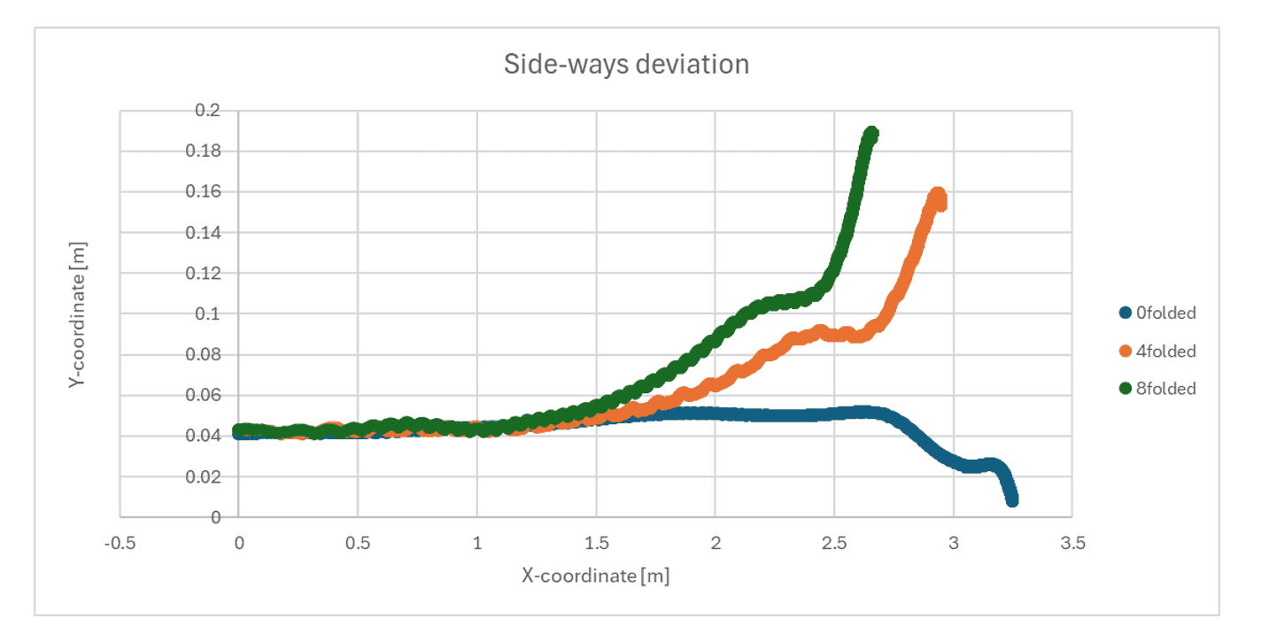
16 feathers are used per shuttle and if the shuttle is too fast for the competition you can be allowed to fold the tip of some feathers. In the picture below you see the geometries used in this study, where 0 or every fourth or every second feather is folded. By running the simulations for folded shuttles we can investigate if the folding impacts the trajectory in any unwanted way, ideally the trajectory looks the same but scaled down so the shuttle moves slower and shorter – but one question that was wanted to get clearer understanding within was if other properties of the trajectory (like the side-way drift due to the Magnus effect) gets affected.
Mesh strategy
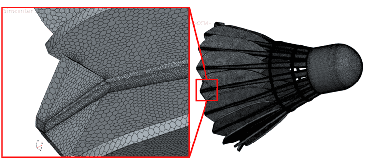
For the surface mesh it is always important to capture the details of the geometry and make sure to have at least two cells across a surface. In the picture below the surface mesh is displayed and also zoomed in at one of the folded feathers.
Moving meshes
Since the shuttle will move across the domain the simulation has to be transient, and a mesh strategy for moving meshes must be used. It is always good to investigate mesh strategy options for your simulation, therefore some different approaches are discussed in this section.
The motion will include both translation and rotation which limits the options for mesh strategies to overset mesh or morphing and remeshing. Morphing and remeshing is better to use when remeshing does not have to occur frequently. Since the shuttle is moving (fast) forward in this case study remeshing would need to occur in every time step, which would be very time consuming, therefore overset mesh is the only viable mesh strategy.
Overset mesh
Following Siemens’ golden rules for overset mesh strategy will get you a long way when it comes to stable overset mesh simulations. You can read more about how to set up your simulations in the blog post via this link, https://volupe.com/simcenter-star-ccm/overset-mesh-in-simcenter-star-ccm/. Additionally, alternate hole cutting was used to ensure a more robust selection of acceptor and donor cells. You enable this feature at the interface.
Overset is the best strategy for predicting the trajectory of a badminton shuttle, but if you have the possibility to choose sliding mesh for example (when you only have rotation, or an axial translation) the other technique is probably less computationally heavy since you would use interfaces instead of interpolation.
Comparison with other strategies for moving meshes
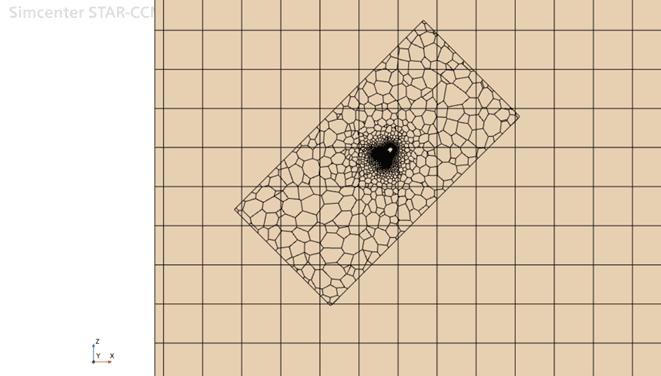
By simulating the pure rotation of the shuttle with a shuttle fix at a certain location, the different moving mesh strategies could be compared.
- Steady flow, MRF
- Transient, sliding mesh
- Transient, overset mesh (same settings as sliding mesh), DFBI
- Transient, overset mesh, DFBI, AMR (for the background mesh)
The simulations showed that overset mesh took much more time than the other approaches, but the rotation of the shuttle was the same. Induced by 60m/s flow from below, the shuttle rotates around 70rps.
This part of the study was carried out to see how well the rotation was captured by overset mesh. It is always good to validate your choice of methods when simulating your real cases.
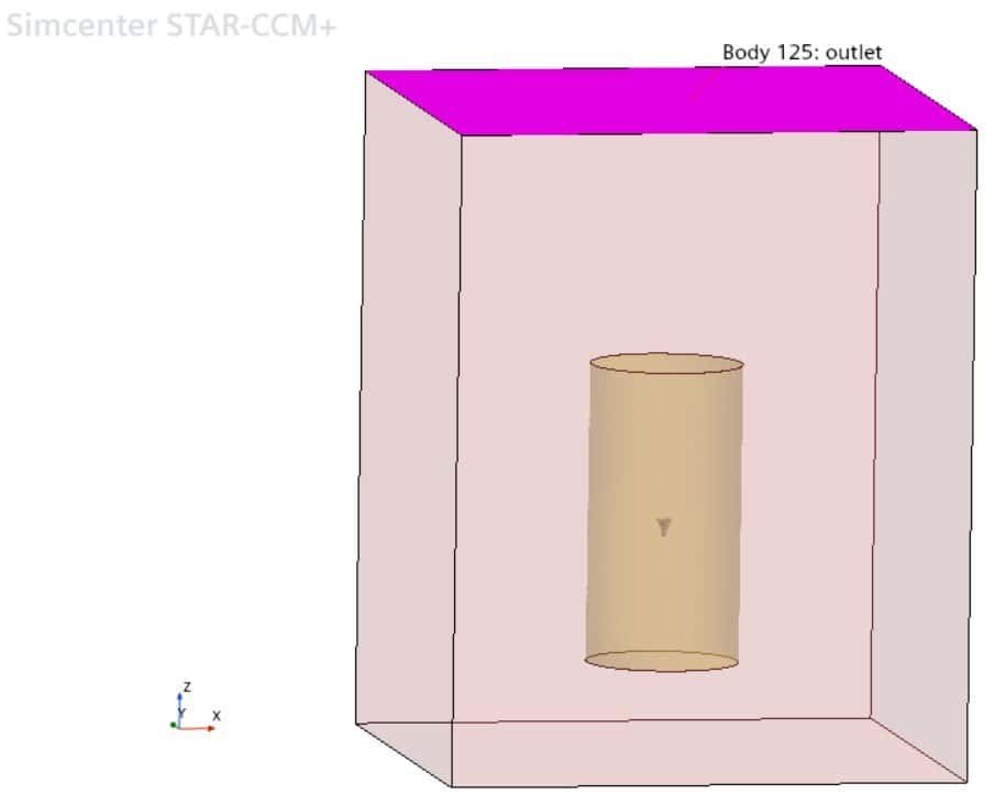
In the picture above the computational domain is visualized with the shuttle pointing downwards and the sliding mesh region (cylinder) is located within a box, where the top surface (behind the shuttle) is an outlet, and all other sides of the box are velocity inlets. Interfaces are set between the subtracted (rotating) cylinder (sliding mesh region in this picture) and the box (steady region). In the MRF simulation the cylinder is not moving and in the overset simulations an overset mesh interface is used instead of subtracting the cylinder from the box.
Refinements
Mesh refinements are important to resolve the gradients in the flow field. Higher gradients require finer mesh, therefore mesh refinement close to the shuttle and behind the shuttle (in the wake region) is required.
Default controls
In Simcenter STAR-CCM+ you set course settings for your region, using default controls, and then you refine the mesh via surface and volumetric controls. For these simulations I have used quite a fine mesh for the surface of the shuttle, and then let the volume cells grow quite fast from the shuttle surface. The overset mesh region has polyhedral cells, and the background mesh has used trimmed (hexahedral) cells with coarse resolution.
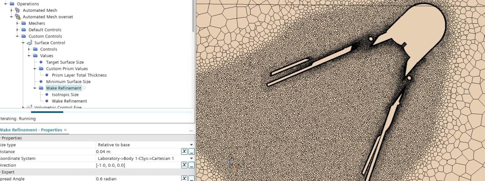
Wake refinements
Wake refinements are possible to set as a surface control, and it was used to get a good resolution of the gradients close to the wall and behind the shuttle. You specify your wake refinement with a spread angle and a distance from the last surface on your object (the feathers in this case), see settings in the picture below.
Adaptive mesh refinement (AMR)
To ensure that the cells in the background mesh are of similar size as the outer cells in the overset mesh region, adaptive mesh refinement was used. It is important to have a smooth transition since the interpolation between the meshes can become less accurate otherwise. For the adaptation, cells were refined if velocity was higher than 4m/s, so cells in the background mesh with higher velocity flow were refined. The refined cells were coarsened when the velocity became lower than 0.2m/s again. Since the movement of the shuttle is the only thing inducing velocity to the fluid this criterion was used. The specific values used for upper and lower limits might be changed in the future to optimize the mesh for these kinds of simulations.
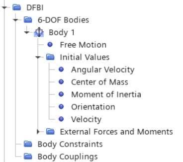
DFBI (Dynamic Fluid Body Interaction)
For objects that move freely in a fluid domain, DFBI bodies are used in Simcenter STAR-CCM+. By adding a new Motion, in Tools, for DFBI translation and rotation, the folder in the picture below appears in the tree structure. For free motions you specify which degrees of freedom you have for your object, in the simulations for the trajectory of a shuttle all degrees are free. In the initial values you specify properties for your object in a coordinate system of your choice.
Coordinate system
Creating local coordinate systems is needed to define DFBI values, since the auto-generated coordinate system for the body is not available to describe DFBI-properties within, since the auto-generated DFBI body coordinate system will follow the object. Therefore you have to create another coordinate system that is independent of the auto-generated coordinate-system for the DFBI body, to specify the initial conditions of the DFBI body, for example Center of mass. Under Tools->Coordinate systems you create local coordinate systems.
Moment of inertia
For badminton shuttles (and many other objects), rotation is a large part of the movement and trajectory. Moment of inertia describes how heavy it is to rotate an object, and this property has been measured and published for badminton shuttles in academic reports.
The values used where [I_xx, I_yy, I_zz] = [1.39E-6, 3.32E-6, 3.32E-6] kg*m^2, with x-axis as rotation axis going through the cork of the shuttle [Lin – 2015 – PhD Thesis].
Chalmers are looking into measuring the moment of inertia with even more precision and are therefore announcing a project to measure this property with two different techniques. So keep your eyes open on the Chalmers project page if this is of interest for you as a student to participate in.
Force
When it comes to force on the DFBI body, gravity is the most important force to include to obtain a physical trajectory. To get the correct starting movement, simulating a serve strike, a function was introduced as an external force. The acceleration of a shuttle when bouncing on the strings of the racquet is very high, additionally the shuttle will turn to fly with the cork first. The turning of the shuttle was not included in the simulations and the impact from the strings was distributed over 5ms to get an acceleration that was possible to simulate in this early state of the investigation of badminton shuttle trajectories.
Solver settings
Choosing solver settings is important since there are models and settings that will allow you to calculate specific phenomena according to best practice. Turbulence models and resolution in time are some of the most important settings, which will be mentioned in this section.
Time step
For time dependent (transient) simulations you must choose a time step that captures the flow phenomena in your real case scenario. One thing that can limit the time step to become low is high velocities of your object. In this simulation the shuttle moves fast in the beginning of the simulation, but since the shuttle rotates very fast after gaining speed this will be the limitation this time. Rotations should be resolved to the extent of one degree of rotation per time step, according to best practice from Siemens in several applications, therefore this is used here as well. Rotating a couple of 10 spins per second (estimated by the simpler CFD setup simulations, together with previous high-speed camera experiments at Chalmers [Johansson et al – 2018 – Behaviour from Eng Point of View]) the time step was set to 5E-5s. The physical time of the shuttle flight (to obtain the full trajectory) is around 1.5s.
Turbulence models
Deciding turbulence model for your simulation can be a difficult decision, since there are many models to choose from and the difference between the models are not always clear. Since one-equation models and two-equation models are less demanding (in terms of mesh resolution and solver time) they are often used in industrial simulations. K-epsilon realizable is commonly used, which gives that there are often simulations to compare with when using this model. If a more academic approach is desired, DES (detached eddy simulations) can be a good choice, since it is not as heavy as LES (large eddy simulations). These two models were therefore used in simulations in this study.
K-epsilon
K-epsilon is a two-equation model, meaning that two parameters are describing the turbulence in the flow. It is also a RANS model, meaning that the model comes from time averaged equations that describes the flow. K-epsilon realizable is the default version of the model in Simcenter STAR-CCM+ and a widely used model in simulation in general. Test data often agrees very well with simulations based on K-epsilon realizable, making it a go-to model for many CFD engineers. Realizability means that restrictions in the model to make it more physically correct are introduced.
DES
DES uses URANS (unsteady RANS) models in the boundary layer (close to the walls) and LES in the bulk flow. Meaning that if the DES model based on K-epsilon is used, then the unsteady version of K-epsilon is used in the boundary layer and then LES is used to predict the flow field in the bulk flow.
In this study DES was used to have a comparison of K-epsilon realizable, to have a more accurate model to compare with. Optimally, the mesh is refined when using LES, but this has not been done yet in this study.
Simulation results
In the results below you see trajectories from the different simulations, together with comments about the results. The three different geometries (non-folded and folded) are used together with different turbulence models and values for moment of inertia.
Trajectories and flow path
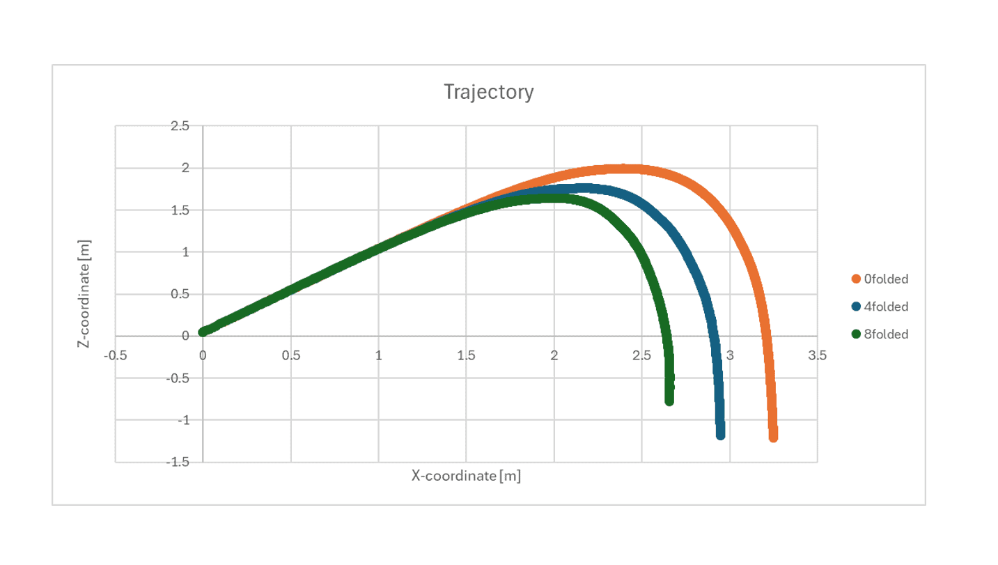
In the picture below the trajectory is visualized from the side, where folding of feathers shows increased drag. This makes the shuttle travelling shorter as more feathers are folded.
Side-ways deviation is visualized in the picture below, where the drift is increased for folded geometries, which would indicate that the Magnus effect is greater in these cases. The side-ways deviation occurs at the end of the trajectory.
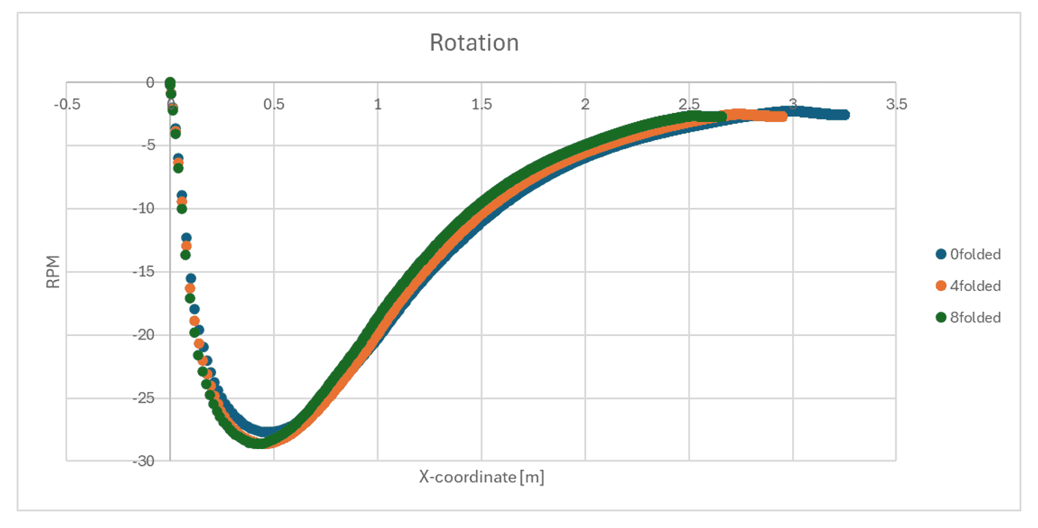
The maximum rotation speed increases with folded geometries, since drag is increased and more force is pushing on the feathers causing the shuttle to rotate. Rotational speed increases and decreases rapidly, but the rotation (measured in rotations per second) is high before the highest point of the trajectory and still several revolutions per second in the end of the trajectory.
Comparisons with different solver settings
A smaller comparison with other solver settings was also carried out. The geometry without folded feathers was run with DES as turbulence model instead of k-epsilon. Another simulation with k-epsilon and moment of inertia set to [I_xx, I_yy, I_zz] = [1.15E-6, 2.8E-6, 2.8E-6] kg*m^2 (instead of [I_xx, I_yy, I_zz] = [1.39E-6, 3.32E-6, 3.32E-6] kg*m^2) was run as well to see how sensitive the results are to this parameter. The values used are estimations from Chalmers pre-study tests to the projects they will perform.
DES
The impact of turbulence model had minor impact on the trajectory but a somewhat lower drag was measured, causing the shuttle to reach higher speed.
New moment of inertia
Comparing the lower moment of inertia, which Chalmers estimated, to the moment of inertia from the literature study the rotation of the shuttle reached a higher rate. The distance travelled was a little bit shorter as well.
Post-processing
Visualizing the results is an important part of all projects. In the animation below you see a video created in Screenplay, the built-in tool for video editing in Simcenter STAR-CCM+.
Conclusions
Properties of the shuttle movement that was focused on in this study, were captured well in the simulations. As expected (and previously seen in experiments), folded geometries have a large impact on the trajectory. The numerical settings had less impact on the results. DES requires a finer resolved mesh than k-epsilon though, which gives that this comparison might need to be re-visited. Higher velocity gives rise to higher rotation rate but how well the Magnus effect is captured will be important to analyze deeper since the non-folded shuttle show almost no side-ways drift (where the expectation is that side-ways drift occur for all shuttles). So, the simulation set up seems to be a good base for further investigation, and some deeper analyses of the simulations already performed.
Future work
This was just the first investigation of badminton shuttle behavior, where more analyzing of the results from this study will be needed to draw more conclusions. There are also many other things that are not taken into consideration, both when it comes to models in Simcenter STAR-CCM+, physics, types of strikes, and how to use the results to innovate shuttles. Some areas that hopefully will be investigated in not too far future are listed below. Stay tuned for further investigations.
FSI (fluid solid interaction)
In this study the geometry of the badminton shuttle is a non-deformable body. This is actually not a good assumption since the shuttle is highly flexible and compressed a lot during the flight. Serve-strikes are not the heaviest strikes though and therefore it was a good choice to begin with investigating. Adding the possibility of deforming the shuttle (due to pressure from the flowing air, or when hitting the shuttle with the racquet) would make the simulations much more demanding though. Therefore, this needs to be validated separately and simulated with high accuracy to get accurate predictions of the flight behavior.
Turing of shuttle (tumbling)
Investigating how the shuttle turns in the air is highly dependent on properties that have been estimated at this point. Moment of inertia is the most important property to have accurately defined, to get an accurate tumbling prediction, and hopefully the upcoming Chalmers project will provide this input. There is also a lot of momentum that has to be transferred correctly from the racquet to the shuttle if the hitting process should be simulated, so getting this part of the trajectory correct will be challenging as well.
Plastic shuttles
In the long-term scope we (Volupe, BWF and Chalmers) hope to being able to define and predict badminton shuttle behavior in such detail so all properties are understood in great detail. With this knowledge the need for real animal feathers could be transferred to plastic feathers with the same properties or at least the same behavior. This would change the industry, so no animals would be needed, the shuttles would break less frequently, and the cost would go down. This would be great in terms of sustainability, so hopefully we can continue the research and development from here.
We at Volupe hope that this blog post was inspiring and gave some relevant insights for your simulations as well. Wishing you all a Merry Christmas and a Happy new year!
Author
Christoffer Johansson, M.Sc.
support@volupe.com
+46764479945