In this week’s blog post we will go over chemistry modelling using reacting species transport in Simcenter STAR-CCM+ with a slight focus towards combustion. This post is the first in a two-part series, where the second one will look at the Flamelet models. We will discuss different models and approaches and when they are valid. As with all modeling we have models available in Simcenter STAR-CCM+ for different regimes. Looking for instance at multiphase simulations we describe regimes using topology, different time, and length-scales. In combustion, or more general chemistry, the regimes we are in often refer to reaction kinetics vs. the turbulence, or more specifically the kinetic timescale and turbulent timescale. We use the term TCI (Turbulence Chemistry Interaction), it refers to accounting for the un-resolved sub-grid heterogeneity within each cell as a result of turbulence and how this heterogeneity affects reaction rate and the resulting species concentrations.

Reaction kinetics

We will start by looking at reaction kinetics and understand the base equation used for chemical reactions. For single or multi-step reactions we use Arrhenius kinetics.

A and B are reactants, C and D are products. a, b, c and d are stoichiometric coefficients of the reactants and products respectively. The rate can then be expressed in modified Arrhenius form as:

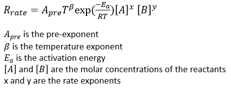
This expression is the basis for many of the reaction models used in Simcenter STAR-CCM+.

Reacting species transport

In reacting species transport we track each individual species in the mechanism of the reaction. Using methane as example the full mechanism can be described using 48 different species and over 200 reactions. When tracking that many species, we solve the transport equations for all of them separately and the effort put on the simulations is very large. Granted there are reduced mechanisms with a limited number of reactions and species that can reduce the number of equations solved, but calculation time still tends to go up. Reaction species transport models are used when the reacting regimes do not fall under Flamelet models, but more on that later. We generally use the reacting species transport modelling approach when in systems where the mixing timescale is shorter than the reaction scale, when the mixing is the predominant limitation to the reactions overall speed.

EBU

EBU or Eddy Break-Up contains a set of models valid when we have fast chemistry, and the reaction rate is determined by the rate at which turbulence can mix the reactants and heat. There are sub-versions of this model. In the Standard EBU model we have completely turbulence driven reactions, the kinetics are too fast to impact overall reaction rate. We assume that when species are mixed, they are immediately burnt. Reaction rate is modeled accounting for turbulent micro mixing. We have the following expressions to describe the rate of fuel depletion. The second expression is used when the option “use product for rate” is activated.

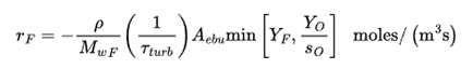
In the above equations we have the parameter A_ebu and B_ebu, and they are tunable coefficients that can be altered to meet experimental data.

In the Hybrid EBU we use the TCI formulation to look at the minimum of turbulence and kinetics, this can vary locally in the system. In the Kinetics only we disregard any effects of turbulence on the reaction rate. This is only valid in laminar flow.

The EBU model is one of the most used models for stable flame conditions, because we can allow for fewer number of reactions, making industrial use cases more feasible. It is however a simplified model with no sub cycling and is suitable for a limited number of reactions that are not stiff. With n number of species, a chemically reacting system has n+1 degrees if freedom, n-1 species concentrations, enthalpy, and pressure of the system. With the n+1 number of quantities we have enough information to solve for all equations in the CFD system. If the number of species is large, the computation can quickly become intensive, hence EBU is suitable for systems with 2-3 reactions. If the system is larger, we use complex chemistry instead.

EBU can be used steady state where the chemistry is calculated over the cell residence time (chemistry time step) and unsteady where the chemistry is calculated over the cell residence time step. It cannot capture complex transient phenomena like lift-off, blow-out, or flame extinction. The EBU model is suitable for non-premixed and partially premixed fuels. It is not suitable for premixed fuels, as we use the assumption that when fuel is mixed it is burnt.

As ignitors for EBU, we can use an EBU ignitor, it forces reaction rates to be mixing limited without using products. We can use a Fixed temperature ignitor which sets the temperature within the ignitor volume shape to a set value.

When analyzing the results in an EBU simulation we should at least look at an overall mass balance, an overall Energy balance and a Species balance. Another good balance to do is an elemental balance of, for instance, the carbon atom.

Thickened Flame

The thickened flame model artificially thickens premixed flame fronts to resolve on the volume mesh. This model is only available for LES simulations and will not be discussed in detail here.

Eddy-contact Micromixing

We can use the Eddy-Contact Micromixing model to do liquid-liquid reactions. Due to the relatively small molecular diffusivity of liquids, the reactions are limited by the rate that reactants can diffuse to the liquid-liquid interface. The Eddy-Contact Micromixing model has the same solution procedure as the EBU model but uses a different method for calculating the turbulent mixing time scale.

Complex chemistry

Aside from EBU, we have the other workhorse of the reacting species transport models, complex chemistry. In for instance burner applications, it is important to understand and be able to predict flame stabilizations and lift-off. When changing the fuel composition flow rate and other operating conditions we need to use a model that can predict details. The complex chemistry combustion model is able to adequately represent the partially premixed region and also get the right auto-ignition information.

The complex chemistry model requires detailed reaction mechanism information about species, reactions, thermodynamics, and transport properties. The properties are best handled and provided using a Chemkin format. The complex chemistry solver uses a stiff CVODE solver for the integration of the chemical source term, meaning that it is capable of handling reaction systems that vary over a large number of time scales.

LFC and EDC

There are two sub models available with the Complex chemistry, the LFC (Laminar flame concept) and EDC (Eddy Dissipation concept). Both of these sub models take the effect of turbulence into account implicitly from the increased turbulent diffusivity provided by the turbulence model selected. The general solution procedure is shown below. The procedure splits the time integration of the chemical state, providing an advantage to the use of reactions with different timescales. The chemical state is integrated in each cell accounting only for the chemical source terms.

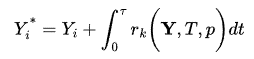
Y denotes mass fractions, r is reaction rate, T is temperature. The species transport equation is then solved with an explicit reaction source term for the species:

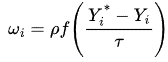
Where the f denotes a mean reaction rate multiplier. The mean reaction rate multiplier is where the LFC and EDC differ. Aside from the implicit turbulence from turbulent diffusivity the EDC mean reaction rate multiplier has an explicit effect from turbulence, it also considers the TCI in the species chemical sources by calculating f from the turbulent timescale:

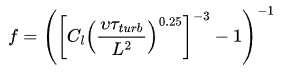
Where C1 is a structure length constant (default 2.1377) and L is the turbulent length scale. In the LFC model the f is set to unity.

In the case of premixed flames, this increased diffusivity results in a flame thickness that is larger than the laminar flame thickness, and a turbulent flame propagation speed that is faster than the laminar flame speed. The flame thickness and speed are controlled through the turbulent Schmidt and Prandtl numbers (set these equal to each other).

Reference case – Sandia flame

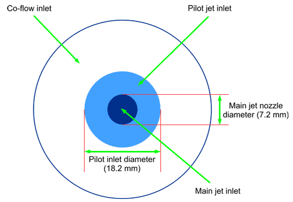
With Simcenter STAR-CCM+ comes a verifications suite that can be accessed and downloaded in the same location on support center where you would download the software. For combustion in general, a common verification case is the Sandia jet flame. It is a well-known setup with reference data available. It was developed by Sydney university and is a methane-air jet flame. In the simulation the geometry is a two-dimensional axisymmetric geometry consisting of the main jet nozzle and the pilot jet inlet. It burns a pre-mixture of 25% methane and 75% dry air by volume. It is shown in the picture below.

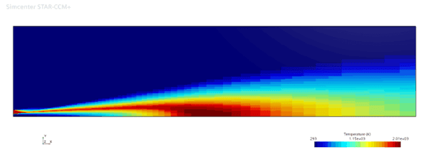
For EBU the hybrid version is used together with standard k-epsilon with high-y+ wall treatment. For comparison we will look at a temperature scalar scene and a temperature plot along the centerline of the simulated result using this method. In the plot the simulated result is compared to the reference, the experimental data.

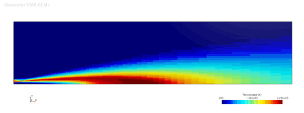
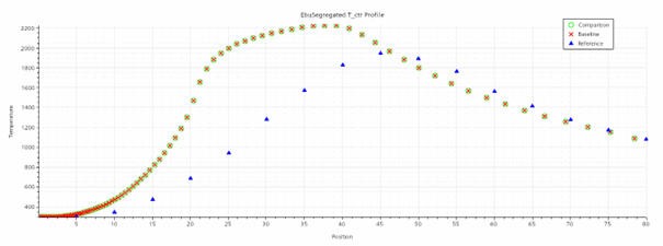
For the Complex chemistry we use Eddy Dissipation Concept (EDC) simulated with Realizable K-Epsilon two-layer model and two-layer all-y+ wall treatment. The equivalent results are shown for this setup as well in the pictures below.

This type of comparison can show, at specific conditions what the different model options can be expected to give. I hope that this has been an interesting read. And stay tuned for the second part of this series coming later this fall, going over Flamelet modeling. As usual, reach out to support@volupe.com with any questions.

Author

Robin Victor
+46731473121
support@volupe.com