Welcome back to our acoustic simulation series. In this week’s blog post we provide guidance for how to set up your simulations in Simcenter STAR-CCM+, and which settings should be used in the GUI.
As mentioned in the previous blog post about acoustics, https://volupe.com/simcenter-star-ccm/capabilities-for-acoustic-simulations-in-simcenter-star-ccm/, the strategy to resolve and obtain accurate results for pressure fluctuations is by first running a RANS simulation and then refine the mesh in order to run a LES simulation. For the RANS compatible acoustic models it is sufficient with a RANS resolution, but generally you will need LES for accurate acoustic simulations.
In this blog post we will therefore focus on how to set up this type of simulation in a user-friendly way. Both post-processing and a discussion about mesh resolution will be covered as well.
Setup of tree-structure in the main GUI
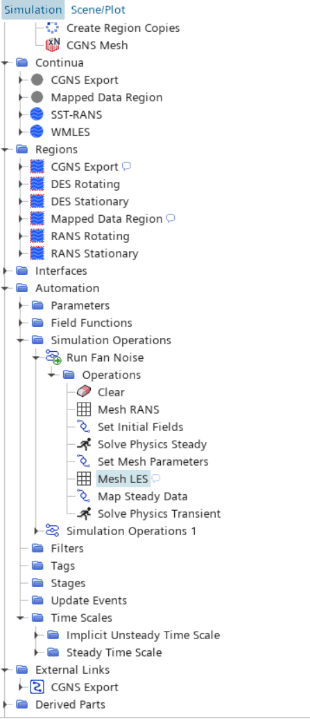
There are several ways to set up the tree-structure in an automated way, for example by using Stages, like in the Siemens Support center article https://support.sw.siemens.com/en-US/product/226870983/knowledge-base/KB000133503_EN_US. This workflow requires only a few steps/clicks compared to other workflows. One alternative workflow is to set up several meshes/regions/continua and map results between them. This approach involves a few additional steps but provides a clearer overview of all available settings. To configure a workflow using data mappers over several regions requires:
- Simulation operation: looping through the setup. Where meshing, choosing which physics is calculated, setting and updating parameters are sequentially changed.
- One mesh operation: Using parameters to setup the refinement levels, which you can update by changing the parameter values in Simulation operations.
- Four continua:
- RANS: for the steady state physics.
- LES: for the transient physical setup.
- CGNS export: result of the external link workflow as described in https://docs.sw.siemens.com/documentation/external/PL20251216891295726/en-US/userManual/starccmp_userguide_html/STARCCMP/GUID-9EC21389-7CAE-4E93-A867-D99F9381968E.html?hl=cgns%2Cexport.
- Mapped data region: to map data.
- Regions: corresponding to all different continua (divided into motion-dependent sub-regions if needed).
- Time scales: to switch between steady and transient physics.
Post-processing the acoustic results
Visualizing the results from an acoustic simulation is preferably done in both the time domain and frequency domain. By finding a good range of pressures to show in a scene, exporting the pictures, creating a movie (or using the export .mp4 file feature directly in Simcenter STAR-CCM+), a video as the example below can be generated.
In the frequency domain the results are preferably visualized as a spectrum. By using a Fast Fourier Transform (FFT) in Tools -> Data set functions -> New -> Point Time Fourier Transform (G[p]), you will have the possibility to read information from a monitor and plot it as a frequency spectrum. The monitor must be set up before the simulation to collect a (maximum) report (pressure) result during the simulation. You update the FFT to use the latest results by right clicking on the monitor symbol for the data set function. In the settings for the FFT you choose which time interval should be used, and which variable the FFT should show. Power spectral density [Pa^2/Hz or dB/Hz] or Sound pressure level are two common variables to visualize for the acoustic performance.
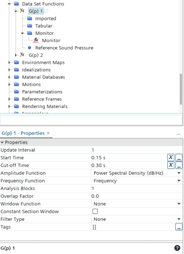
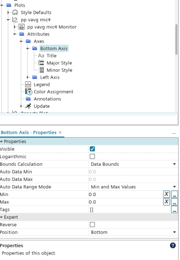
Visualize the spectrum by creating a new empty plot. Right-click to add data, point to the data set function monitor data. In the plot settings for axis, you have the possibility to set logarithmic axis, which is generally used when visualizing sound pressure level for example.
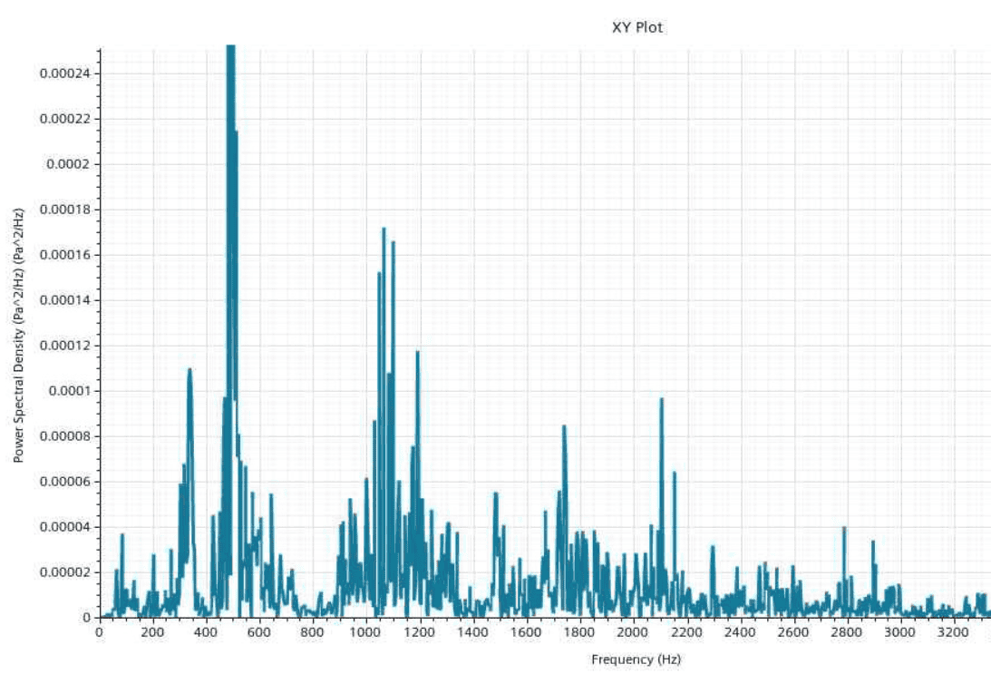
Below you find a visualization of the frequency spectrum for a typical fan simulation. The blade passing frequency is around 500Hz which is (by far) the highest peak in the spectrum. To visualize that there are several peaks in the spectrum the plot is cut, meaning that the actual peak for the frequency around 500Hz is beyond the height of the Power spectral density in the plot.
Mesh study for acoustic simulations for fans
The requirements for mesh resolution are high for LES simulation (https://support.sw.siemens.com/en-US/product/226870983/knowledge-base/KB000033594_EN_US and https://support.sw.siemens.com/en-US/product/226870983/knowledge-base/KB000037975_EN_US), it is therefore interesting to investigate how fine mesh you actually need to obtain good acoustic results. A mesh study was carried out to analyze the effect of grid resolution for the acoustic results. The meshes generated had 6, 12, 18, 75 or 167 million cells. In the picture below you see overviews of the mesh closest to the fan for all simulations (a zoomed-out picture for the 75million cell mesh as well), in order to get a feeling for which resolutions were compared in the mesh study.
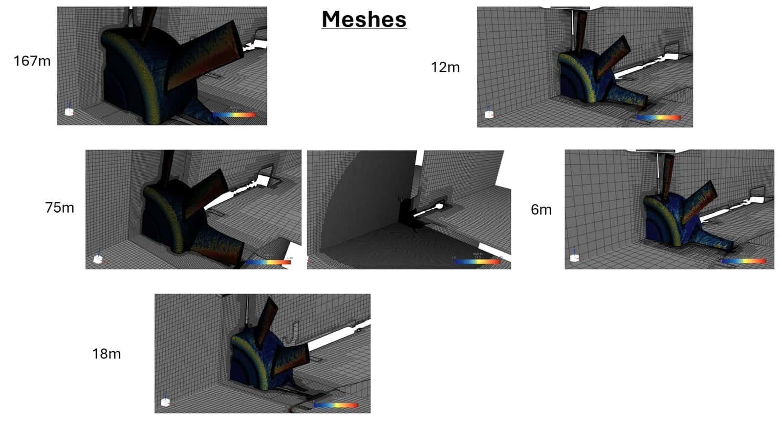
Also remember the best practice for noise calculations can be found here (follow this link for best practice for noise calculations https://support.sw.siemens.com/en-US/product/226870983/knowledge-base/KB000040408_EN_US), which also includes choices for mesh type etc.
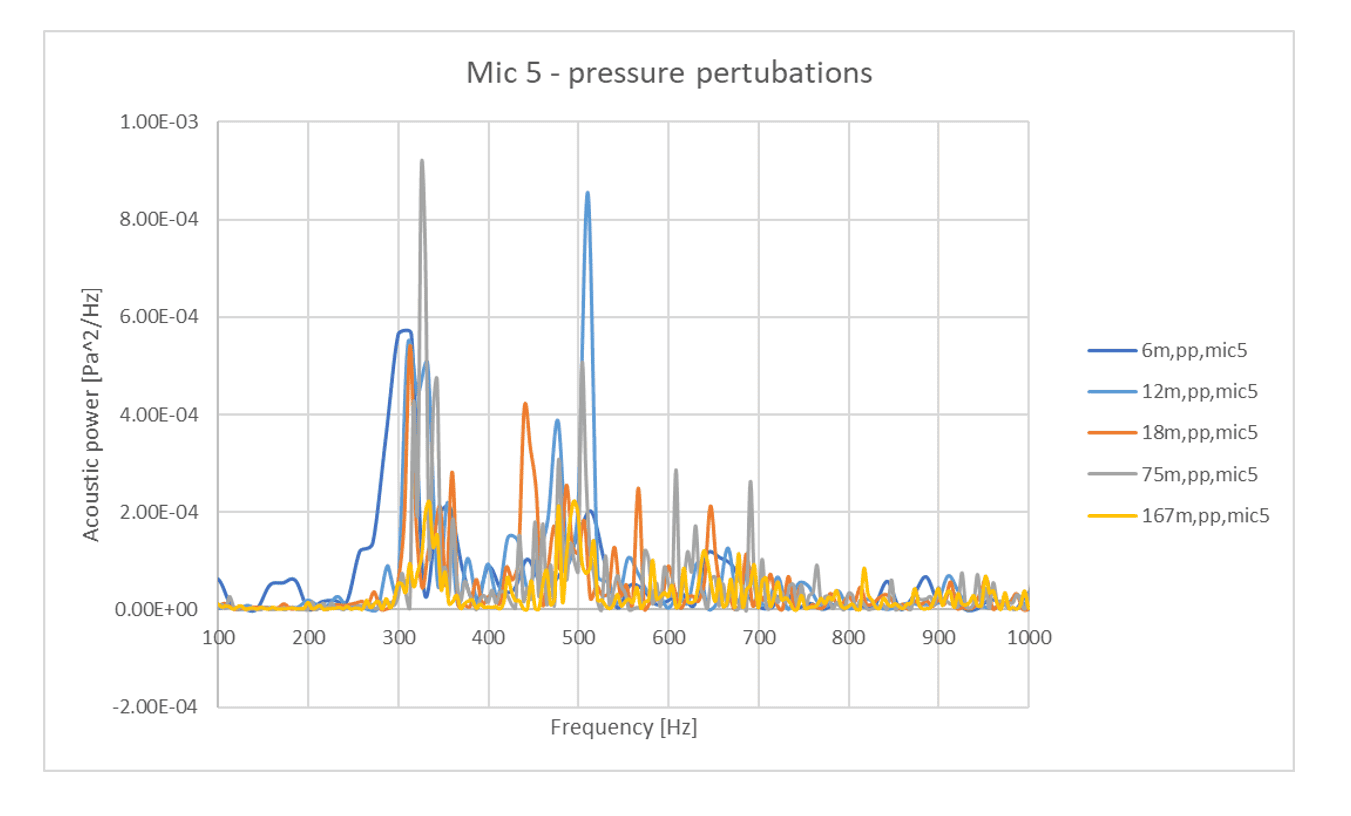
When it comes to acoustic results, the pictures below visualize how the data varies dependent on how many cells was used, where the majority of cells were spent to resolve the volume around the fan (as seen in the picture above). Both for power spectral density and acoustic power the results get better with fine mesh, but the trend is still showing even with coarser mesh. Concluding that you will obtain useful results even if your mesh resolution is lower than required LES resolution, but for accurate results you will need fine resolution.

Summary and conclusions
The idea with this blog post is to describe a setup that match the criteria for Siemens’ best practice for acoustic simulations, especially for rotating fan simulations. Mesh resolution is directly coupled to the accuracy of your results, and the settings should be chosen carefully. For visualization the FFT functionality via data set functions is very useful, together with visualization for the actual pressure fluctuations.
Additional solver settings to consider are:
- Double precision (R8) version needed
- Calculate the cell size and time step based on Taylor micro scales
- Interfaces using Close Adjacent Cells are recommended
- Speed of sound definition needs to be set (continua/gas/”your fluid”/materialProperties/speedOfSound)
- Convection scheme MUSCL 3rd-order/CD (continua/segregatedFlow)
- 2nd order time scheme (solvers)
Thank you for reading our blog post, we hope that this information will be useful in your everyday work. Please reach out to us at support@volupe.com if you need any assistance with your simulations.
Author
Christoffer Johansson, M.Sc.
support@volupe.com
+46764479945