In this week’s blog post we are looking into acoustic capabilities and models in Simcenter STAR-CCM+. Since there are several models for acoustic applications it is important to understand their differences and when to choose which model. We will describe the models by starting with the least computational expensive one and then go to more accurate models, but first we start with some general information and theory.
General guideline
Sound propagation originates from small pressure fluctuations within the fluid. To resolve these pressure fluctuations, it typically required to have both fine mesh resolution and a small time steps. The frequency range that humans can hear is from 20Hz to 20kHz. The highest level of accuracy (Direct noise calculations) does therefore (at least) require LES resolution of the mesh, to resolve all frequencies of pressure fluctuations. There are several models to help you obtain results even though you cannot afford to simulate with LES accuracy, but then you have to keep in mind that you are introducing significant approximations into the simulation. This includes both mesh resolution and simulating at least 20 time steps per fluctuation within a cell. Meaning that higher frequencies will require more computational power.
Since obtaining results from these kinds of detailed transient simulations are computationally demanding, there are recommendations on how to ensure the workflow being as efficient as possible. The recommended workflow for running acoustic simulations starts with running steady state RANS simulations on a coarse mesh, and when the mean flow is calculated a time dependent URANS should be calculated. This simulation will be the initial condition for your LES simulation, but please note that the LES simulation requires a finer mesh resolution and therefore remeshing is needed before your acoustic results can be calculated. The simulation provides information about the pressure fluctuations and from monitors the results can be presented in either the time domain or the frequency domain. Pressure levels will be reported from the time domain and frequency spectrum (by performing a FFT analysis) it is possible to extract from the frequency domain.
Note: Acoustics is a topic that requires high fidelity simulations and therefore it is recommended to always run acoustics simulations in double precision (R8-version of Simcenter STAR-CCM+), even though some models can be used accurately in the mixed precision version.
Theory about sound generation
In aeroacoustics, sound sources are commonly classified as monopoles, dipoles, and quadrupoles. These source types correspond to different physical mechanisms of sound generation in fluid flows.
A monopole represents a source of fluctuating mass or volume, such as a pulsating body or mass injection. It radiates sound uniformly in all directions and is the simplest and most efficient acoustic source. A dipole arises from fluctuating forces acting on the fluid, typically due to interactions between a flow and solid boundaries (e.g., lift and drag fluctuations on an airfoil). Dipole sources are directional and exhibit a characteristic figure-eight radiation pattern. A quadrupole is associated with turbulence within the flow itself, originating from fluctuating Reynolds stresses without requiring solid surfaces. These sources produce more complex radiation patterns and are generally weaker at low flow speeds but dominate in high-speed turbulent flows, such as jet noise.
Broadband noise
Broadband noise is a RANS model and will therefore be less computational heavy than the other models available in Simcenter STAR-CCM+. This model is used for near-field noise predictions to determine the location and strength of the acoustic source.
The models Curle and Proudman are available for 3D simulations. Curle model evaluates the local acoustic power of dipole noise sources (generated per unit surface) and Proudman model evaluates quadrupoles (generated per unit volume). The two models are possible to run in parallel. Both models assume isotropic turbulence.
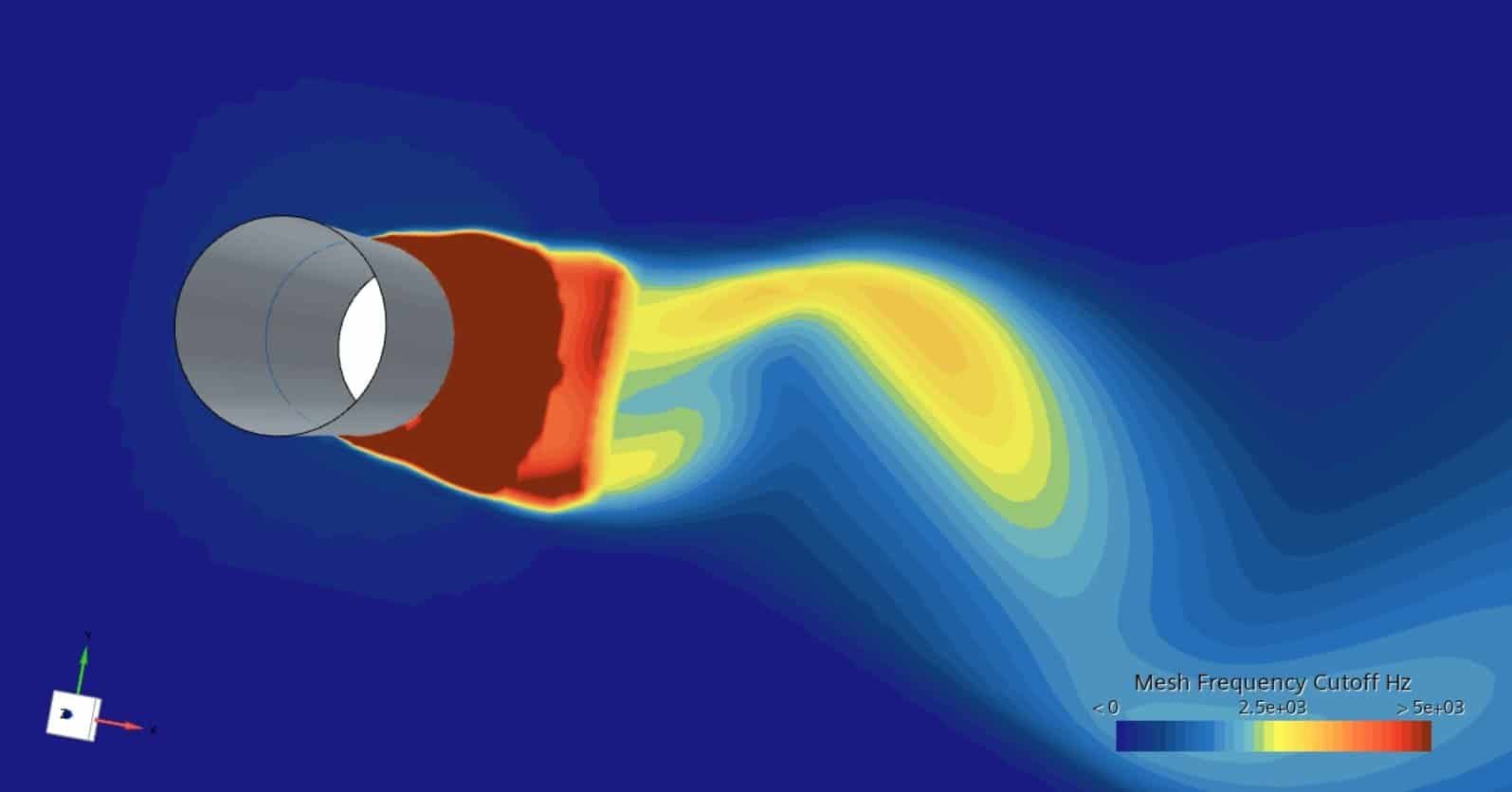
The finer mesh resolution you have in your simulation the higher frequencies are possible to capture. In the picture below, the mesh frequency cut-off field function is displayed to show which frequencies are captured at specific locations. The wake refinement close to the cylinder is finer and therefore even (above) 5kHz can be captured, while the coarser mesh downstream captures frequencies around 2.5kHz.
Ffowcs Williams-Hawkings (FW-H) model
The FW-H model captures far-field noise by setting up microphones (surface or receivers) that are activated when the model is selected. The location of the microphones should be far from the source of sound. One limitation of FW-H is that reflection from walls is not taken into account, meaning that walls are not affecting the information that transfers between the noise source and the microphone. Simulations where this model is suitable are therefore large open domains where the sound is generated by turbulence around an airfoil or an airplane.
FW-H is compatible with other models and can therefore be used in combination with mode complex models to obtain the far field noise as well as the local pressure fluctuations.
There are two types of FW-H strategies, On-The-Fly FW-H and Post FW-H model. You need to select one of these strategies in the continua in order to activate FW-H. Post-model used information that has been stored in a .simh file and will therefore be used in a post-processing step after the simulation is completed. On-The-Fly FW-H will provide a prediction for quadrupoles along with that the simulation is running. FW-H is available in both steady state and unsteady simulations.
Acoustic wave model
The Acoustic Wave model uses the theory of Acoustic perturbation equations (APE) to predict the noise generated by the fluid flow. The Acoustic Wave solver is one-way coupled with the flow solver through this APE-based noise source term and models the acoustic pressure field inside a specified zone of interest.
When you use the Acoustic Wave model, it is recommended that you also activate the Cell Quality Remediation model.
Note: The acoustics wave solver is not compatible with non-stationary regions, for example fans and other rotating (or translating) applications.
Lighthill wave model
The Lighthill Wave model provides an efficient method to model sound generation and propagation for incompressible fluid flow (Ma < 0.2).
To calculate the sound propagation in turbulent flows, the Lighthill Wave model introduces a separate wave equation to separately track pressure perturbations. This perturbation is called Lighthill pressure, which is the sum of acoustic pressure and hydrodynamic pressure.
Perturbed convective wave model
The idea behind PCW is to try finding dipole-pressure, like the flow in a turbulent boundary layer, and classify the pressure perturbations. Similar to the Lighthill wave model, PCW uses a separate wave equation to calculate the sound generation and propagation in incompressible fluid flows. However, this wave equation solves for an acoustic potential, from which the acoustic pressure can be derived. Additionally, the model provides a pressure perturbation field, which represents a combination of acoustic pressure and hydrodynamic pressure. The Perturbed Convective Wave model is intended for studying the noise everywhere in the flow domain, irrespective of the magnitude of turbulent flow fluctuations. For noise predictions in regions where the hydrodynamic pressure is negligible, the computationally less expensive Lighthill wave model provides reasonable results. However, in regions where turbulent fluctuations are dominant, only PCW, which directly solves for the acoustic pressure, can provide insight into the sound field.
Since the model supports transient flow, wall reflection and non-stationary regions, this model is the most advanced model available before moving to Direct noise calculations.
Sponge layer modelling
The sponge layer method is available to dampen outer boundary conditions effect on your acoustics simulations. Unsteady aeroacoustics simulations require effective non-reflective boundary conditions to prevent spurious reflected acoustic waves from the boundaries of the computational domain interfering with the aero-acoustic results. By specifying the sponge layer thickness at the Sponge layer model in the continua you obtain a damping zone for the outlet boundaries.
The sponge layer model can be used in combination with the other simulation methods. And in addition to this strategy, for wall boundaries the possibility of acoustic dampening in terms of non-reflecting boundaries can be set at boundary level in the regions.
Direct noise calculations
Direct noise calculations are the most accurate way we can simulate sound propagation, and that means resolving pressure fluctuations to the level of 0.01Pa. The best practice from Siemens available at the Support center goes deeper into the requirements for this workflow:
https://support.sw.siemens.com/en-US/product/226870983/knowledge-base/KB000040408_EN_US
Note: Lighthill wave model and PCW are not compatible with Ideal gas. This means that in order to account for compressible effects Direct noise calculation is the only option.
Acoustic modal analysis
The Acoustic modal analysis model available in Simcenter STAR-CCM+ allows you to simulate acoustic mode shapes, frequencies, and linear growth rates. This model predicts standing wave shapes, frequencies, and linear stability.
Coupling to Simcenter 3D with vibro-acoustics
Since Simcenter STAR-CCM+ does not simulate sound propagation with solids (this needs to be performed in the frequency domain), vibro-acoustics is performed in Simcenter 3D (Siemens software for FEM simulations). The recommended workflow is therefore to couple the fluid simulations from Simcenter STAR-CCM+ to Simcenter 3D via mapping data (surface pressure) on to the walls and perform co-simulations using both software.
Summary
There are many models to choose from, and which one to use comes down to what you are trying to simulate and learn from your simulations. From steady state simulation, looking at frequency spectrum, modelling the sound, to resolve the pressure fluctuations with the fluid – everything is possible to simulate in Simcenter STAR-CCM+. To get even better understanding about acoustics and how to simulate sound propagation with Simcenter STAR-CCM+ we highly recommend looking into the Siemens tutorials available in the documentation:
If you want to dig deeper into the capabilities for the acoustic models, they are also described in the documentation:
Theory behind the acoustic models can be found in the documentation as well:
This blog post is a first description of the models available in Simcenter STAR-CCM+. There will be a follow-up in this blog post to bring some light on specific settings and comparing simulation results to experimental results. The recommended workflow will also be described more in detail in this blog post. So, keep on following our blog and if you have any questions – you are always welcome to reach out to support@volupe.com.
Author
Christoffer Johansson, M.Sc.
support@volupe.com
+46764479945