Tangential plotting along a circular line in Simcenter STAR-CCM+

Johan BernanderSenior Application Specialist
In short
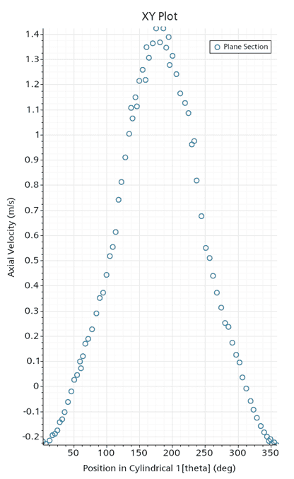
Simcenter STAR-CCM+ has no derived part for a curved line, but intersecting derived parts make one. In a cylindrical duct, a Cylinder Section of 0.1 m radius cut by a Plane Section gives a circle; plotting against theta in a cylindrical coordinate system shows, for example, axial velocity versus angle.
Plotting along a line can be done easily in Simcenter STAR-CCM+ using a Line Section or Line Probe derived part, but these derived parts are limited to straight lines. Imagine instead that you want to plot field data along a curved line, e.g. as a function of angular position. For this scenario there is no native derived part to be used, so you need to be a bit creative to achieve this. In this blog post we will demonstrate how to get it done.
Demonstration case
To demonstrate the workflow we will use a dummy case where we induce a recirculation flow inside a cylindrical duct. The geometry is a 1 meter tall cylinder with a radius of 0.15 meters. An air flow is introduced in the bottom of the cylinder with an inclination angle of roughly 26.5 degrees, creating a recirculation pattern inside the cylinder.
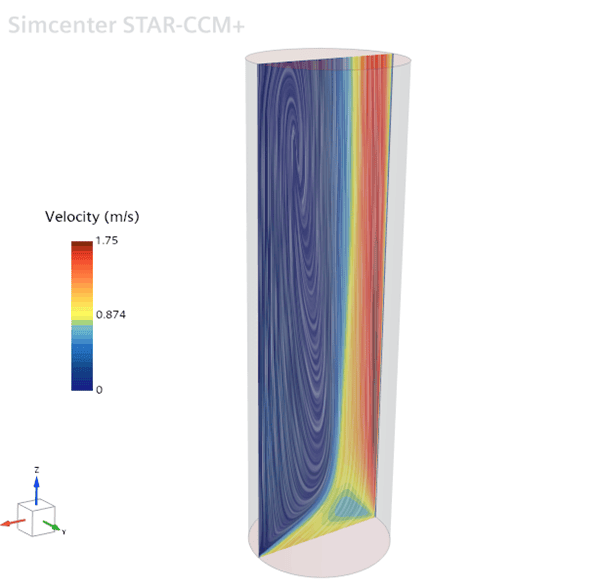
Step 1 – Creating a cylindrical coordinate system
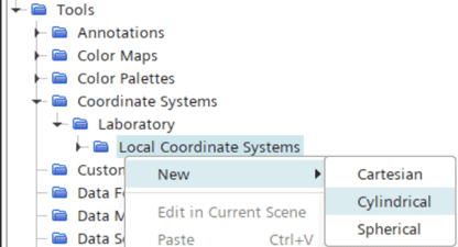
If we want to use angular position as our input variable, we need to establish this variable (theta) by creating a cylindrical coordinate system. This is done under Tools -> Coordinate Systems -> Laboratory -> Local Coordinate Systems.
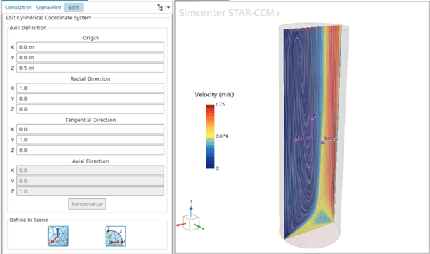
In this particular case we decide to place the origin in the middle of the cylinder, i.e. at [0, 0, 0.5] meters. We let the X-axis define the radial direction, and the Y-axis define the “plane” where our angular coordinate, theta, will vary. Consequently, the Z-axis defines the axial direction. The coordinate system setup can be seen below.
Step 2 – Creating a line with intersecting derived parts
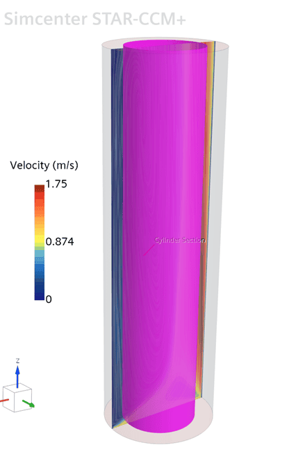
Since there is no native derived part for creating a curved line in Simcenter STAR-CCM+, we need to find another way of doing this. In this case we will utilize the fact that two (or more) intersecting parts create lines along the intersection(s). Here we want a circular line, so we start by creating a Cylinder Section derived part.
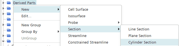
We let the cylinder run through the entire tube, with a radius of 0.1 meter.
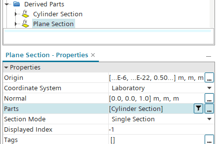
Now we need an intersecting part to create a line. Here we decide that we want our line in the center of the tube, so we create a horizontal Plane Section at Z = 0.5 meters. To create an intersection, we let our Cylinder Section derived part be the input part to the horizontal Plane Section.
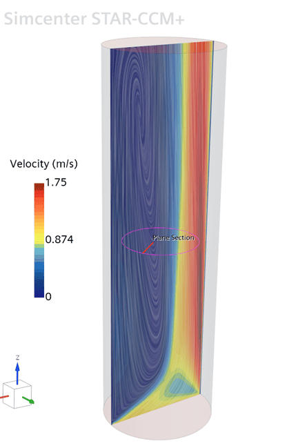
The resulting derived part is the circular line we sought to achieve, see below:
Step 3 – Create a plot
Now we have all the input needed to create our tangential plotting. We go to Plots and create a new XY Plot.

Right-click the XY Plot and select Add Data.
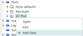
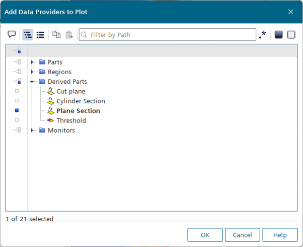
In the dialog window, select the Plane Section we just created, then click OK.
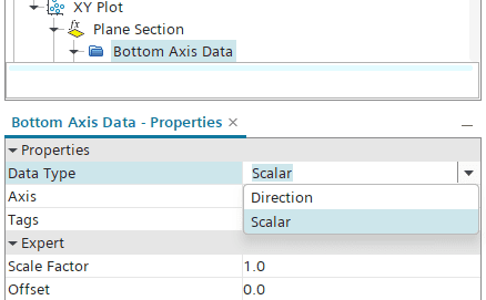
Go to the Bottom Axis Data and set the Data Type to Scalar.
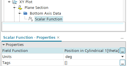
Then set the Field Function to Position in Cylindrical 1 [theta] to use the angular position as the input variable.
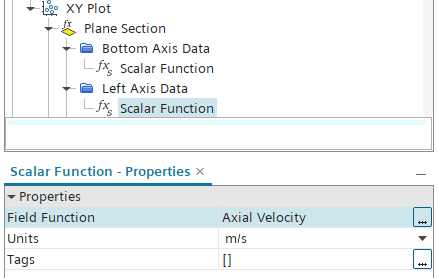
Now we can analyze a property of choice along the angular position on the circular line, e.g. axial velocity, and select it as input for the left axis. Now we can analyze a property of choice along the angular position on the circular line, e.g. axial velocity, and select it as inputfor the left axis data.
The resulting plot in this case will look like this:
Final remarks
In the example above we used derived parts only to create our plotting curve. Please note however, that you could also intersect Part Surfaces and/or Boundaries to create curves or lines of interest.
I hope that you found this demonstration useful. As always, reach out to support@volupe.com if you have any questions or comments.