Moody chart and pipe pressure drop calculator
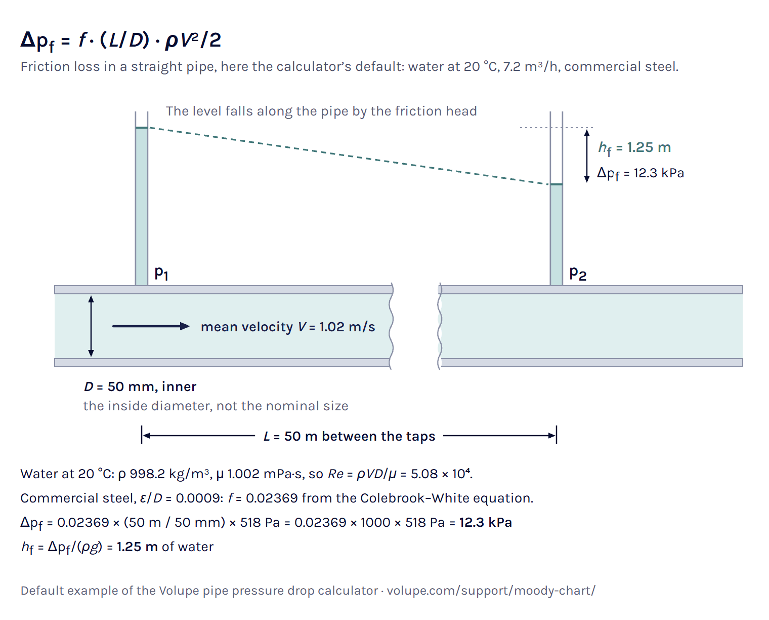
Pipe pressure drop on a live Moody chart, set to 7.2 m³/h of water in 50 m of 50 mm steel.
Calculator
The Darcy–Weisbach equation
The Darcy–Weisbach equation gives the pressure drop from wall friction in a straight pipe running full, for any liquid and in laminar as well as turbulent flow [1, 2]:
Δp = f (L/D) ρV2/2 (1)
Here f is the Darcy friction factor, L the length, D the inner diameter, ρ the density and V the mean velocity, the volume flow divided by the flow area πD2/4 [1]. D is the inner diameter of the pipe, not the nominal pipe size [3]. ρV2/2 is the dynamic pressure, so the pipe loses fL/D times the dynamic pressure over its length.
In the case the calculator opens with, 7.2 m³/h of water at 20 °C in a 50 mm pipe, V = 0.002 m³/s / 1.963 × 10⁻³ m² = 1.019 m/s and ρV2/2 = 998.2 × 1.0192/2 = 518 Pa. With f = 0.02369 and L/D = 1000, the 50 m pipe loses 0.02369 × 1000 × 518 Pa = 12.3 kPa.
Note that Δp is a loss of mechanical energy. In the energy equation between two sections (the Bernoulli equation with a loss term) it is the loss term [1]. Between two points of one pipe at the same height, it equals the drop in static pressure. Height is left out here. If your outlet is Δz higher than the inlet, add ρgΔz, 9.79 kPa per metre for water at 20 °C.
USBR traces the equation to Darcy’s formula of 1857, as modified by Weisbach and others [4]. Because it holds for any liquid, we use it here rather than the Hazen–Williams formula, which has no viscosity term and was developed for water in turbulent flow [2].
For a gas, (1) assumes a constant density, which only holds while the pressure drop is small compared with the absolute inlet pressure. CIBSE and the sources quoted in NBS Technical Note 356 put the limit at 10 % of it [5, 6]. Above that, the arithmetic mean of the inlet and outlet densities agrees more closely with the compressible result than the inlet density does, and NBS TN 356 calls it the modified-incompressible formula [6]. For drops above 40 % Crane calls for a method that includes the compressibility of the gas [7].
In the compressed-air example, 360 kg/h of air at 20 °C and 7 bar gauge in 50 m of 25 mm galvanised pipe, the result is the isothermal compressible solution [6], 158 kPa, which is 19.7 % of the absolute inlet pressure of 8.01 bar and puts it in the middle band. You get that solution at every pressure ratio, since it tends to the result of (1) as the drop gets small. The mean density comes within 1 % of it, while (1) with the inlet density alone gives 141 kPa, about a tenth too low (our calculation).
Load the compressed-air example in the calculator ↑
Head loss
Head loss is the same loss written as a height of the fluid, in metres: the mechanical energy lost per unit weight [1]. The head loss formula follows from (1):
hf = Δp/(ρg) = f (L/D) V2/(2g) (2)
With standard gravity, 9.80665 m/s² [11], the 12.3 kPa of pipe friction in the opening case is a head loss of 1.25 m of water, and the fittings add 0.15 m. You get both forms in the result.
Non-circular ducts
For a duct that is not round, use the hydraulic diameter Dh = 4A/P (flow area A, wetted perimeter P) in place of D [12], and give the flow as the mean speed from the real area, because a volume flow would be divided by the area of a circle. The approximation is about 15 % off near the start of turbulence, better at higher Re, and poor, about 40 %, in laminar flow [13]. The Pipes and ducts section of the Reynolds number calculator shows how to find Dh.
How to read the Moody chart
The Moody chart, or Moody diagram, plots the Darcy friction factor f against the Reynolds number Re, with one curve for each relative roughness ε/D, on logarithmic axes [14, 15]. Moody published it in 1944 as a simple way to estimate f for the head loss in clean, new pipes running full with steady flow [16]. Its curves are the laminar law f = 64/Re and the Colebrook–White equation [15], and the chart is a way to solve them by eye.
To read it by hand, work out Re = ρVD/μ and ε/D, follow the curve labelled with your ε/D on the right (interpolating between two printed ones) to your Re on the bottom axis, and read f on the left [14]. At Re = 10⁵ and ε/D = 0.001 that gives about 0.022, where the Colebrook–White equation gives 0.02217. The DOE handbook reads 0.04 at Re = 40 000 and ε/D = 0.01 [17], where the equation gives 0.03936, so that reading is 1.6 % high (our calculation).
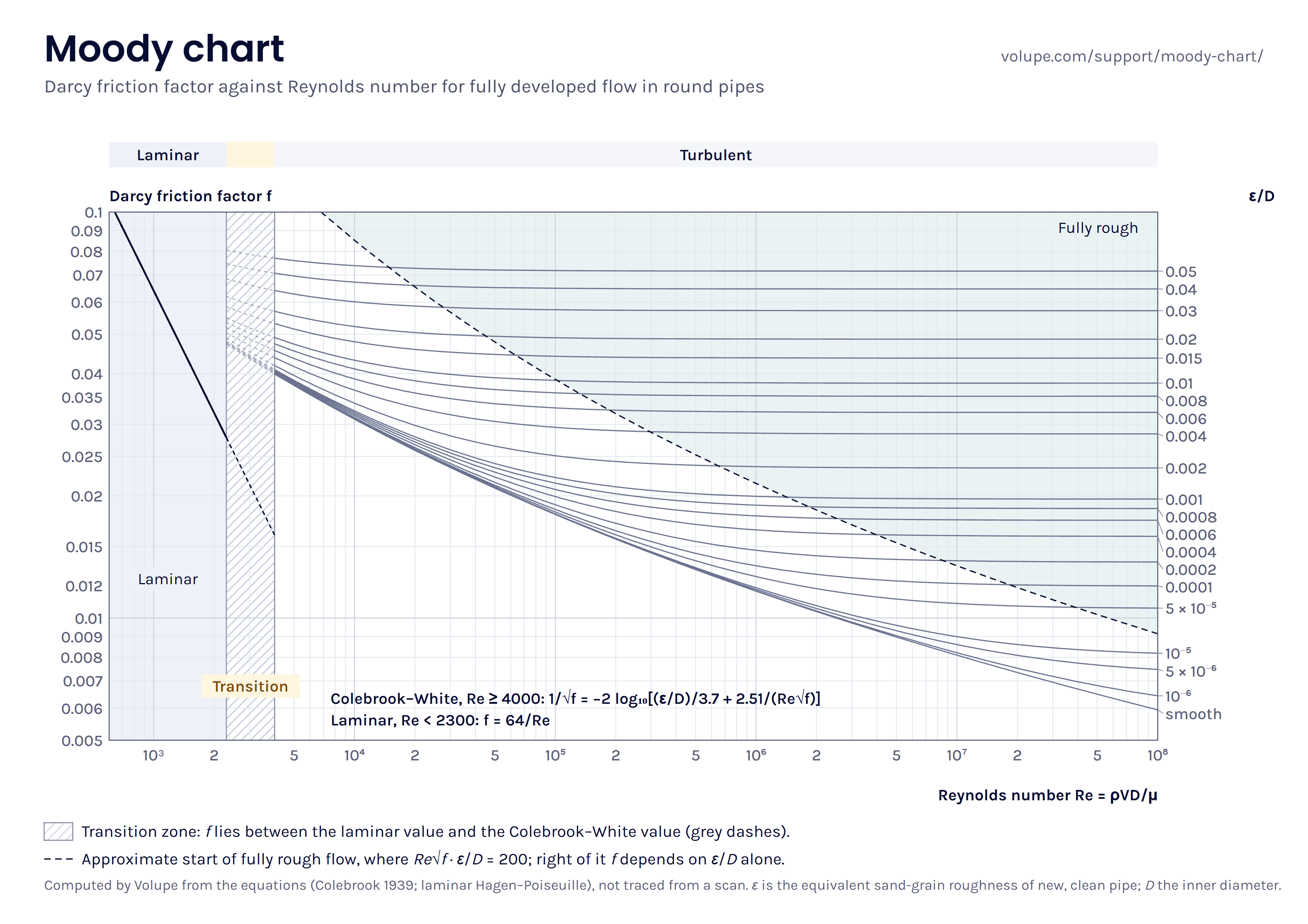

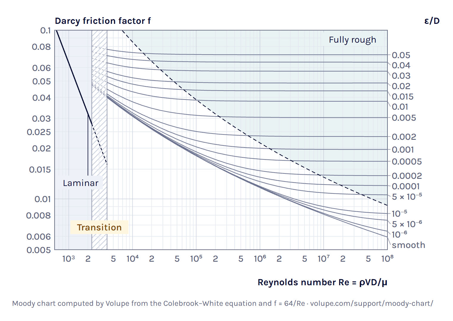
Here you see your pipe’s own ε/D curve over the standard ones, with the point at your Re and f and the reading on both axes. Drag the point and the flow and Δp follow it. Under Download chart you get the same chart without a pipe on it, as an SVG file or an A4 image for printing.
Load the Moody reading example in the calculator ↑
Laminar flow: f = 64/Re
In fully developed laminar flow the friction factor follows exactly from the Hagen–Poiseuille solution [12]:
f = 64/Re (3)
On the log–log chart it is the straight line on the left, and roughness does not enter. Put (3) into (1) and the density drops out, Δp = 32μLV/D2, so the laminar pressure drop rises in proportion to the flow and, at a given flow, falls with the fourth power of the diameter.
In the laminar example, 0.5 L/min of water at 20 °C in a 10 mm drawn tube, Re = 1057.44, well inside the laminar range, so f = 64/Re and the 10 m tube loses 340 Pa.
The transition zone
Between laminar and turbulent flow there is no single friction factor. Moody left this zone hatched, without definite curves, and called f there indefinite, giving initial turbulence, imperfections in the pipe, noise and pressure waves as the likely reasons [18]. Any value between the laminar and the turbulent curve can be obtained [18], and CIBSE calls the pressure drop there unpredictable [5].
In a smooth pipe in transition, laminar stretches and turbulent puffs and slugs travel together, each with its own friction law, so the average f lies between the two values, weighted by the share that is turbulent [18]. Roughness hardly moves the start. Nikuradse found it between 2160 and 2500 for all his sand-roughened pipes [19].
You get the same pipe limits as in the Reynolds number calculator. Below Re 2300 the flow counts as laminar, since that is the top of the range where turbulence only appears as local puffs [20]. From 4000 it counts as turbulent, a round limit above the 3000 where pipe flow is usually turbulent [21]. In between, f and Δp come as a range from 64/Re up to the Colebrook value carried below 4000, and we take the upper end as the design figure, since it is the conservative one. For 1.4 L/min of water at 20 °C in the same 10 mm tube, Re = 2960.8 and f = 0.02162 to 0.04383, a factor of 2.03, and the 10 m tube loses 0.952 to 1.93 kPa.
Other methods put one number in the gap: EPANET a cubic fitted to the Moody diagram between 2000 and 4000 [2], Churchill’s 1977 correlation a smooth curve [14], and Simcenter Flomaster, a 1D network code, a linear blend of its laminar and turbulent values across 2000 to 4000 [22]. For the same tube Churchill gives 0.0429, inside the range (our calculation).
Load the transition example in the calculator ↑
Fully rough flow
At high Reynolds numbers the curves level off. The Colebrook term with Re becomes small, and f depends on ε/D alone [1]:
1/√f = −2 log10[(ε/D)/3.7] (4)
Nikuradse called this the range of the quadratic law [19]. With f constant, (1) makes Δp rise with the square of the velocity, so twice the flow costs four times the pressure. In the concrete-main example, 2 m³/s of water at 20 °C in 1000 m of 1000 mm concrete pipe, Re = 2.54 × 10⁶, and twice the flow gives 3.99 times the pressure drop.
We draw the dashed line where Re√f·ε/D = 200, where f has come within about 2 % of its fully rough value. The constant is our choice, checked against the dashed line on the Moody chart in Çengel and Cimbala [14]. For the default pipe, ε/D = 0.0009, it lies at Re ≈ 1.60 × 10⁶, about 30 times the flow you start with. That pipe is between smooth and fully rough.
Darcy friction factor: the Colebrook–White and Haaland equations
The Darcy friction factor f is the dimensionless factor in the Darcy–Weisbach equation (1) that carries the wall friction. In laminar flow it depends on Re alone, through (3), and in turbulent flow on Re and the relative roughness ε/D [12], where the Colebrook equation is an accepted informal standard [23].
The Colebrook equation
The Colebrook equation, also called the Colebrook–White equation, is the turbulent part of the Moody chart [15, 24]:
1/√f = −2 log10[(ε/D)/3.7 + 2.51/(Re√f)] (5)
Colebrook published it in 1939, joining the smooth-pipe and rough-pipe laws of Prandtl, von Kármán and Nikuradse in one formula fitted to his own measurements on commercial pipes [25]. With ε = 0 it is the smooth-pipe law, and as Re grows it tends to (4) [1, 25]. It is accepted for Re from 4000 to 10⁸ and ε/D up to 0.05 [23], and outside that you get a warning.
f appears on both sides, so (5) has to be solved by iteration. We use Newton’s method on 1/√f, started from Haaland’s value. On 100 000 random combinations of Re and ε/D it needed one to four steps to settle in the last digit of a double-precision number. It reproduces the 15-digit values Praks and Brkić published, such as f = 0.038630738574792 at Re = 3 × 10⁴ and ε/D = 0.009 [23], and it agrees with Clamond’s method, a two-step iteration that converges to machine precision [26].
The physics is not that exact. The constants 2.51 and 3.7 were fitted to measurements, and the formula itself is not very accurate [26]. Measurements on commercial steel pipe in Princeton’s Superpipe showed a much more abrupt change from smooth to rough than Colebrook’s, and a fully rough pressure drop at least 13 % below what Colebrook gives with the roughness usually assumed [27]. Clamond’s reason for solving it accurately anyway is that a crude solution can make simulations hard to repeat [26].
Explicit approximations: Haaland and Swamee–Jain
Explicit formulas give f in one step. Two of them are the Haaland equation, from 1983 [1],
1/√f = −1.8 log10[((ε/D)/3.7)1.11 + 6.9/Re] (6)
and the Swamee–Jain equation, from 1976 [1]:
f = 0.25/[log10((ε/D)/3.7 + 5.74/Re0.9)]2 (7)
Maurer gives the Haaland equation as within 1.5 % of Colebrook [1], and a 2011 statistical review found it the most suitable explicit formula for hand calculation [25]. Over the whole chart, Re from 4000 to 10⁸ and ε/D up to 0.05, we found it within about 1.4 % of Colebrook–White, at most 1.4 % low around Re 9 × 10⁴ and up to 1.3 % high in a smooth pipe at both ends of the chart, Re 4000 and 10⁸. It is within 1 % on 87 % of our grid.
Swamee–Jain is the form EPANET uses above Re 4000 [2]. It is within 1 % on 89 % of our grid, but near the lower turbulent limit it runs high, up to 3.4 % at Re 4000, and it is within 2 % only from about Re 12 000 (our calculation). That is more than the 2 % in Cimbala’s course notes [24].
You see both beside the Colebrook value with the difference in per cent, never as the answer, and not below Re 4000, where neither applies. At Re = 10⁵ and ε/D = 0.001, Colebrook gives 0.02217, Haaland 0.02197 (−0.9 %) and Swamee–Jain 0.02234 (+0.8 %).
Darcy or Fanning friction factor?
Two friction factors are in use, and they differ by a factor of four. The Darcy factor of the Moody chart and of (1) is four times the Fanning factor, which is the wall shear stress divided by the dynamic pressure. In laminar flow that makes f = 64/Re in one and 16/Re in the other [12].
Check which one a correlation, a spreadsheet or a solver report uses before you compare values. Our page on dimensionless numbers lists the Fanning friction factor with its definition, and Compare with your result flags a typed f close to a quarter of the Colebrook value as a likely Fanning factor.
Relative roughness and pipe roughness values
Relative roughness is the absolute roughness ε of the pipe wall divided by the inner diameter, ε/D. In turbulent flow f depends on that ratio rather than on ε itself [12], so the same material is relatively rougher in a small pipe. New commercial steel with ε = 0.045 mm is ε/D = 0.0009 in a 50 mm pipe and 9 × 10⁻⁵ in a 500 mm one.
The ε in the tables is an equivalent sand-grain roughness: the size of the uniform sand in Nikuradse’s experiments that gives the same friction as the real wall [19, 26]. It is not a height you can measure on the wall. Colebrook and White showed that real, uneven roughness behaves differently from uniform sand between smooth and rough [26], and the Moody chart uses Colebrook’s curves for commercial pipe [15].
The values are for new, clean pipe, and roughness can change a lot with age [2]. Wichowski and co-workers measured ε = 27.6 mm in 150 mm cast-iron water mains after 30 years, against 0.9 mm for their new pipe, itself above the value in the table [29]. If you have a measured pressure drop for an old line, put it into Compare with your result. The curve it lands on is the roughness the pipe behaves as.
The sources agree on steel, galvanised iron and cast iron. They disagree most on concrete: 0.3 to 3 mm in the Purdue notes and EPANET, 0.9 to 9 mm in Çengel and Cimbala [2, 14, 28]. For a material with a range you get the result for the value in the table, and where the range moves Δp by more than 1 % the chart draws it as a band. In the concrete-main example, 0.3 to 3 mm moves Δp from 49.3 to 84.9 kPa around the 63.9 kPa of the 1 mm value.
Minor losses and K values
Entrances, exits, bends, tees and valves each cost a pressure drop of their own, written as a loss coefficient K times the dynamic pressure, with V the mean velocity in the pipe. The losses add to the pipe friction [3]:
Δp = (fL/D + ΣK) ρV2/2 (8)
The name minor losses can mislead, because in a short system the fittings can cost more than the pipe [1, 17]. In the opening case, a sharp-edged entrance (0.5), four flanged 90° elbows (0.3 each), an open gate valve (0.2) and an exit into a tank (1.0) make ΣK = 0.5 + 4 × 0.3 + 0.2 + 1.0 = 2.9, which is 2.9 × 518 Pa = 1.50 kPa, 10.9 % of the total. The same loss can be given as an equivalent length of straight pipe, Leq = ΣKD/f [17], here 2.9 × 0.05 / 0.02369 = 6.12 m.
Treat any table K as a typical value. Published values for the same fitting type differ widely [3], and tests of fittings of one type from different manufacturers differed by 2 to 161 % [32]. Where a manufacturer gives K for the valve you use, take theirs [31]. K also depends on the Reynolds number [32] and rises at low Re, which Hooper’s 2-K method models [33]. You get a warning when there are fittings and Re is below 10 000, a threshold we chose.
Two rows depend on how the pipe ends. The exit loss of 1.0 is the velocity head lost into a tank [31], while a free jet to atmosphere has no exit loss, because the velocity leaves with the jet [30]. In laminar flow the exit into a tank costs two velocity heads, since the exit K equals the kinetic-energy factor α [30], which is 2 for the parabolic profile.
Catalogue K values are measured on single fittings with long straight pipe on both sides. In Rahmeyer’s tests on steel and iron elbows, elbows at least 20 diameters apart did not affect each other, and elbows closer than that lost less than the sum of their single values, so for elbows close together the summed K is usually on the safe side [32]. It is not a rule for every combination. Fabian Hasselby’s post on flow interaction between components compares two bends placed close together in Simcenter Flomaster, with its Component Interaction option, and in Simcenter STAR-CCM+. There the sum looks conservative for a U-bend, while an S-shaped pair loses more than the U-bend.
Worked example: water in a steel pipe
This is the case you see when the page opens, worked through by hand: water at 20 °C and 1 atm flowing at 7.2 m³/h through 50 m of commercial steel pipe with a 50 mm inner diameter, from one tank to another, with a sharp-edged entrance, four flanged 90° elbows, an open gate valve and an exit into a tank.
Properties. The water model gives ρ = 998.2 kg/m³ and μ = 1.002 mPa·s [8, 9], and commercial steel has ε = 0.045 mm [14, 28].
Velocity and Reynolds number. Q = 7.2/3600 = 0.002 m³/s and A = π × 0.052/4 = 1.963 × 10⁻³ m², so V = 1.019 m/s and Re = 998.2 × 1.019 × 0.05 / 0.001002 = 5.08 × 10⁴, well above 4000, which makes the flow turbulent.
Friction factor. ε/D = 0.045/50 = 0.0009. Newton’s method on (5), started from Haaland’s 0.02340, reaches f = 0.02369 in three steps. On the chart the point lies just below the 0.001 curve and well left of the dashed line, where both terms of (5) count.
Pipe and fittings. (1) gives 0.02369 × 1000 × 518 Pa = 12.3 kPa for the pipe. The fittings have ΣK = 2.9 and add 2.9 × 518 Pa = 1.50 kPa.
Total. Δp = 12.3 + 1.50 = 13.8 kPa, or 1.41 m of head loss, and 89.1 % of it is pipe friction. If the second tank sits higher than the first, the lift comes on top.
Checks. The entrance length, about 4.4Re1/6D = 1.34 m, is short against 50 m, and the fully developed f is a fair assumption [13]. The hydraulic power to push the water through, before pump losses, is ΔpQ = 27.5 W.
Double the flow to 14.4 m³/h and the pressure drop becomes 51.2 kPa, 3.7 times as much. It is less than four times because f falls from 0.02369 to 0.02180 as Re doubles, and in fully rough flow it would be four times. The Pipe diameter mode answers the reverse question: in the sizing example, 30 m³/h through 100 m of commercial steel with the same fittings and at most 50 kPa, it finds an inner diameter of at least 75.8 mm.
From one pipe to a pipe network
Here you work on one pipe at a time. In a network the flow divides between parallel branches until every branch between the same two junctions loses the same pressure, so no branch can be worked out on its own.
Simcenter Flomaster solves such networks in 1D. A pipe there has length, diameter and absolute roughness among its inputs, and its fittings, bends and valves carry loss data based on D. S. Miller’s Internal Flow Systems [22, 34]. Its default pipe friction uses an explicit approximation of the Colebrook–White equation, so for one straight pipe in turbulent flow the two should agree closely [22]. By our comparison its formula has the form of the Swamee–Jain equation (7), up to 3.4 % above Colebrook near Re 4000 and within 1 % over most of the chart.
Where bends and valves sit closer together than the long straight runs their K values assume, Flomaster can correct the loss coefficients for the interaction [22], as in Fabian’s post above. It can also work backwards: you give the flow each branch needs, and it works out the component data that deliver it, such as an orifice size or a valve opening [22, 34]. Our post on flow balancing in Simcenter Flomaster sizes the orifices of a sprinkler system that way.
When a valve closes fast or a pump trips, a steady answer is not enough. Flomaster’s transient solver follows the pressure surge, or water hammer, through elastic pipes with the method of characteristics, which is why it asks for the wave speed in each pipe [22, 35]. Our post on incompressible transients in Simcenter Flomaster shows the set-up.
Inside one part, such as a valve body or a manifold, 3D CFD gives the flow and its pressure drop directly. In Simcenter STAR-CCM+ the Pressure Drop report compares the mass-flow-averaged absolute total pressure on two groups of boundaries, usually the inlet and the outlet [36]. With gravity on, that pressure holds the hydrostatic part, computed with the reference density [36]. Between boundaries at different heights the report therefore includes the hydrostatic pressure difference as well as the flow losses. Christoffer Johansson’s post shows it in a model you can download.
To check such a result here, take a straight run of constant diameter, far enough from bends for the flow to be fully developed [13, 14], and type its pressure drop or friction factor into Compare with your result. It appears on the chart as a second marker, with the difference from Colebrook–White in per cent.
References and changelog
References
[1] E. Maurer, Hydraulics and Water Resources: Examples Using R, Santa Clara University, 2024, chapter 4, Water flowing in pipes: energy losses (CC BY-NC 4.0). edm44.github.io
[2] L. A. Rossman et al., EPANET 2.2 User Manual, EPA/600/R-20/133, U.S. Environmental Protection Agency, 2020, chapter 3, The Network Model: Pipes, and table 3.2. epanet-manual.readthedocs.io
[3] Hydraulic Institute, Data Tool, Fluid Flow III-B, Frictional losses in valves, fittings and bends (from the Engineering Data Book, 2nd edition, 1990), equation 3.A.6 and table 3.B.1. datatool.pumps.org
[4] U.S. Bureau of Reclamation, Friction Factors for Large Conduits Flowing Full, Engineering Monograph No. 7, 1965, revised 1977. www.usbr.gov
[5] CIBSE Guide C: Reference data, Chartered Institution of Building Services Engineers, 2001, sections 4.6.2 and 4.7.1. www.cibse.org
[6] J. Hord, Comparison of incompressible flow and isothermal compressible flow formulae, NBS Technical Note 356, National Bureau of Standards, 1967. nvlpubs.nist.gov
[7] Crane Co., About TP-410, the publisher’s summary of Crane Technical Paper No. 410, Flow of Fluids through Valves, Fittings and Pipe. tp410.com
[8] IAPWS R7-97(2012), Revised Release on the IAPWS Industrial Formulation 1997 for the Thermodynamic Properties of Water and Steam. iapws.org
[9] IAPWS R12-08, Release on the IAPWS Formulation 2008 for the Viscosity of Ordinary Water Substance, 2008. iapws.org
[10] U.S. Standard Atmosphere, 1976, NOAA, NASA and USAF, NASA-TM-X-74335 (Sutherland constant S = 110.4 K). ntrs.nasa.gov
[11] A. Thompson and B. N. Taylor, Guide for the Use of the International System of Units (SI), NIST Special Publication 811, 2008 edition, appendix B.8. nvlpubs.nist.gov
[12] NPTEL course 112104118, Fluid Mechanics, IIT Kanpur: lecture 26, Losses and friction factors, and lecture 35, Concept of friction factor in a pipe flow. archive.nptel.ac.in
[13] F. Stern, ME:5160 Intermediate Mechanics of Fluids, chapter 6 part 1, Viscous flow in ducts, University of Iowa, notes of fall 2023 (file of 2025). stern.lab.uiowa.edu
[14] J. M. Cimbala, Major head losses, turbulent, ME 320 lesson 08E, Penn State University, with figure A-12 (the Moody chart and its roughness table) of Y. A. Çengel and J. M. Cimbala, Fluid Mechanics: Fundamentals and Applications, 4th edition, McGraw-Hill. www.me.psu.edu
[15] P. R. de Souza Mendes, A note on the Moody diagram, arXiv:2308.10360, 2023. arxiv.org
[16] L. F. Moody, Friction factors for pipe flow, Transactions of the ASME 66(8), 671–678, 1944 (abstract). doi:10.1115/1.4018140
[17] U.S. Department of Energy, DOE Fundamentals Handbook: Thermodynamics, Heat Transfer, and Fluid Flow, volume 3, DOE-HDBK-1012/3-92, 1992, Fluid flow: head loss, and table 1. www.energy.gov
[18] R. T. Cerbus and T. Mullin, Completing Moody’s friction diagram in the turbulent transitional regime, arXiv:2110.14966, version 3, 2024. arxiv.org
[19] J. Nikuradse, Laws of flow in rough pipes, NACA Technical Memorandum 1292, 1950 (translation of VDI-Forschungsheft 361, 1933). ntrs.nasa.gov
[20] V. Mukund and B. Hof, The critical point of the transition to turbulence in pipe flow, Journal of Fluid Mechanics 839, 76–94, 2018. doi:10.1017/jfm.2018.31
[21] W. Moebs, S. J. Ling and J. Sanny, University Physics Volume 1, OpenStax, Rice University, 2016, section 14.7 Viscosity and turbulence. openstax.org
[22] Simcenter Flomaster documentation, version 2504, Siemens Digital Industries Software: User Guide, Getting Started and Components Reference Manual.
[23] P. Praks and D. Brkić, Advanced iterative procedures for solving the implicit Colebrook equation for fluid flow friction, Advances in Civil Engineering 2018, 5451034. doi:10.1155/2018/5451034
[24] J. M. Cimbala, Fully developed pipe flow equations, ME 320 handout, Penn State University, 2012. me.psu.edu
[25] S. Genić, I. Arandjelović, P. Kolendić, M. Jarić, N. Budimir and V. Genić, A review of explicit approximations of Colebrook’s equation, FME Transactions 39(2), 67–71, 2011. simlab.mas.bg.ac.rs
[26] D. Clamond, Efficient resolution of the Colebrook equation, Industrial and Engineering Chemistry Research 48(7), 3665–3671, 2009. doi:10.1021/ie801626g
[27] L. I. Langelandsvik, G. J. Kunkel and A. J. Smits, Flow in a commercial steel pipe, Journal of Fluid Mechanics 595, 323–339, 2008 (abstract). doi:10.1017/S0022112007009305
[28] C. Wassgren, Pipe flows: head losses, ME 30800 lecture notes, Purdue University, 2016, with the ME 309 formula sheet. engineering.purdue.edu
[29] P. Wichowski et al., Hydraulic and technological investigations of a phenomenon responsible for increase of major head losses in exploited cast-iron water supply pipes, Water 13(11), 1604, 2021. doi:10.3390/w13111604
[30] Y. A. Çengel and J. M. Cimbala, Fluid Mechanics: Fundamentals and Applications, 4th edition, McGraw-Hill, table 8-4 (loss coefficients), as reproduced in J. M. Cimbala, Pipe flow minor losses, ME 320 lesson 08F, Penn State University. www.me.psu.edu
[31] R. S. Subramanian, Minor losses, CH 330 course notes, Clarkson University. web2.clarkson.edu
[32] L. Lin, M. Duarte Batista and N. Milesi Ferretti, State-of-the-art review on measurement of pressure losses of fluid flow through pipe fittings, NIST Technical Note 2206, National Institute of Standards and Technology, 2022. doi:10.6028/NIST.TN.2206
[33] V. Fester, P. Slatter and N. Alderman, Resistance coefficients for non-Newtonian flows in pipe fittings, chapter 7 in Rheology, InTech, 2012 (the Hooper 2-K method). doi:10.5772/34199
[34] Siemens Digital Industries Software, Early design of thermo-fluid systems, Simcenter product page, read 2026. www.siemens.com
[35] A. Deponti, What’s new in Simcenter Flomaster 2019.1, Siemens Simcenter blog, 2019. blogs.sw.siemens.com
[36] Simcenter STAR-CCM+ documentation, version 2606, Siemens Digital Industries Software, 2026: Pressure Drop report, Pressure field functions and Gravity.
Changelog
November 2026: first published, with the calculator, the Moody chart and this guide. Each cited statement was checked against the saved text of its source, which for Crane is the one sentence quoted from its own summary of Technical Paper No. 410, and the Simcenter Flomaster and Simcenter STAR-CCM+ statements against the Siemens documentation. Comparisons marked “our calculation” are our own.
Questions about the Moody chart
Questions about pipe losses, fittings or a network model? We reply within one day.
Ask a technical question →
How do you calculate the Darcy friction factor?
In laminar flow, below Re 2300, the Darcy friction factor is f = 64/Re. In turbulent flow, from Re 4000, solve the Colebrook–White equation, 1/√f = −2 log₁₀(ε/(3.7D) + 2.51/(Re√f)), by iteration, or use an explicit formula such as Haaland’s, which is within 1.5 % of it. You need the Reynolds number Re = ρVD/μ and the relative roughness ε/D. Between Re 2300 and 4000 there is no single value: f lies somewhere between the laminar and the turbulent one. The Moody chart calculator above does this for you and shows the result on the chart.
What is the Moody chart?
The Moody chart, also called the Moody diagram, is a log–log chart of the Darcy friction factor f against the Reynolds number Re, with one curve for each relative roughness ε/D. Moody published it in 1944 as a simple way to estimate friction factors for the head loss in clean, new pipes. On the left is the laminar line f = 64/Re, in the middle the transition zone, and to the right the turbulent curves of the Colebrook–White equation, which level off where the flow becomes fully rough.
What is relative roughness?
Relative roughness is the absolute roughness ε of the pipe wall divided by the inner diameter D. In turbulent flow the friction factor depends on ε/D rather than on ε, so the same material is relatively rougher in a small pipe. New commercial steel has ε = 0.045 mm, which gives ε/D = 0.0009 in a 50 mm pipe. The ε in roughness tables is an equivalent sand-grain roughness, not a measured height, and it is for new, clean pipe.
What does head loss mean?
Head loss is a pressure loss given as a height of the flowing fluid: the mechanical energy lost in the flow per unit weight of fluid, h = Δp/(ρg). For water at 20 °C a head loss of 1 m is 9.79 kPa. In the energy equation between two points of a pipe, it is the loss term that the ideal Bernoulli equation leaves out.
When does the Darcy–Weisbach equation not apply?
The equation itself holds for any liquid in laminar or turbulent flow. The limits come from the friction factor and from assuming a constant density. Take care with a gas whose pressure drop is more than about 10 % of the absolute inlet pressure, with two-phase flow, with non-Newtonian fluids, with short pipes where the flow is still developing, in the transition zone between Re 2300 and 4000, and above Re 10⁸ or ε/D 0.05, where the Colebrook equation is extrapolated.
How do I convert a Fanning friction factor to a Darcy friction factor?
Multiply it by four. The Darcy friction factor, used in the Moody chart and in Δp = f(L/D)ρV²/2, is four times the Fanning friction factor, which is the wall shear stress divided by the dynamic pressure. In laminar flow the Darcy factor is 64/Re and the Fanning factor 16/Re. A friction factor about a quarter of the Moody chart value is usually a Fanning factor, so check which one a correlation or a solver report uses before you compare.