Reynolds number calculator

Calculate the Reynolds number of a pipe or duct flow, a flat plate, a cylinder or a sphere, with air and water properties at your temperature, and read the flow regime for that shape with the limits the sources give.

Free calculator and guide · 23 min read · Updated October 2026

Reynolds number formula

The Reynolds number equation (1) gives the ratio of the inertial forces in a flow to the viscous forces [1]. Here ρ is the density of the fluid (kg/m³), U the flow speed (m/s), L a characteristic length (m), μ the dynamic viscosity (Pa·s) and ν = μ/ρ the kinematic viscosity (m²/s).

Whether your flow is laminar or turbulent depends on Re, on the shape and on what the flow has met upstream.

Which length to use

A regime limit only holds for the length it was given for. That is the inner diameter D of a circular pipe, not the nominal pipe size, and the hydraulic diameter D_h of any other duct (see Pipes and ducts). A flat plate uses the distance x from the leading edge, which gives the local Re_x, and a cylinder or a sphere in a free stream its diameter. For anything else, such as a wing or a vehicle, use the length that the data you compare with are based on, and say which one you used.

Dynamic and kinematic viscosity

Data sheets give the viscosity in two forms. The dynamic viscosity μ is in Pa·s, often as mPa·s or centipoise (1 cP = 1 mPa·s), and the kinematic viscosity ν = μ/ρ in m²/s, often as mm²/s or centistokes (1 cSt = 1 mm²/s = 10⁻⁶ m²/s) [2]. Water at 20 °C has μ = 1.002 mPa·s and ν = 1.003 mm²/s [3, 4], two numbers that look almost the same. Air at 20 °C and 1 atm has a dynamic viscosity 55 times lower than water, μ = 1.813 × 10⁻⁵ Pa·s, but a kinematic viscosity 15 times higher, ν = 1.506 × 10⁻⁵ m²/s. This means that at the same speed and size, air gives you a Reynolds number 15 times lower than water.

The usual slip is a kinematic viscosity typed in cSt with m²/s selected, which makes Re a million times too small, or a kinematic viscosity typed into the μ field. The calculator checks for both and offers you the fix in one click.

How the calculator gets the fluid properties

Air is dry air as an ideal gas, ρ = p/(RT), with R = 287.12 J/(kg·K) from Lemmon et al. [5], and its viscosity follows Sutherland’s law, μ = 1.716 × 10⁻⁵ (T/273.15)^1.5 (273.15 + 110.4)/(T + 110.4) Pa·s with T in kelvin [6]. We compared it with the reference equation of Lemmon and Jacobsen [7]. It is within about 1 % from −50 to 150 °C, about 2 % off at 300 °C and about 5.5 % at 1000 °C, where the reference data themselves differ by about as much [7, 8]. At 1 atm the ideal-gas density is within 0.1 % of the reference equation from 250 to 1000 K and 0.16 % low at −50 °C, and the error grows with pressure, to 1.6 % at 10 bar and −50 °C [5]. Above 10 bar the calculator still computes but warns that you need real-gas properties, and below 0.01 bar it points you to the Knudsen number instead. Humidity is left out. At 20 °C and 50 % relative humidity it lowers the density by about 0.4 %, small next to the spread of any transition Reynolds number.

Water uses the IAPWS standards, IF97 for the density [4] and the 2008 formulation for the viscosity [3], for liquid water from 0 to 350 °C. The default pressure is 1 atm, and above 100 °C you give a pressure above the boiling pressure, at least 198.7 kPa at 120 °C [4]. From 0 to 100 °C the viscosity is within 0.3 % and the density within 0.05 % of the saturated-water table in Çengel and Cimbala [8]. The sea water option is ITTC standard sea water, fixed at 15 °C, with ρ = 1026.0 kg/m³ and ν = 1.189 × 10⁻⁶ m²/s [9]. For any other fluid, type ρ and μ, or ν alone.

How to calculate the Reynolds number

Take the case the calculator opens with, water at 20 °C flowing at a mean speed of 1 m/s through a pipe with an inner diameter of 25 mm. With ν = 1.0034 × 10⁻⁶ m²/s, equation (1) gives Re = UD/ν = 1 × 0.025 / (1.0034 × 10⁻⁶) = 2.49 × 10⁴, or about 24 900. The density form gives the same number, Re = ρUD/μ = 998.2 × 1 × 0.025 / (1.0016 × 10⁻³) = 2.49 × 10⁴.

Flow at this Reynolds number is turbulent in any ordinary pipe. Laminar flow at 2.49 × 10⁴ has only been kept in experiments built to keep disturbances out [10]. If you want laminar flow in this pipe, stay below about 2000, where turbulence dies out on its own [11, 12]. Here that means a speed below about 0.08 m/s.

The units cancel, as you can check on the density form. ρUL has the units kg/m³ × m/s × m, and μ has Pa·s, which is kg/(m·s), so the ratio is a pure number [2]. Re is dimensionless, and it comes out the same in SI and US units as long as you convert every input consistently.

Laminar vs turbulent flow

In laminar flow, sometimes called streamline flow, the fluid moves in layers that slide past each other without mixing. Turbulent flow mixes the layers through eddies and swirls, with velocities across the main direction of flow, and it resists the flow more [13]. Which one you get depends on the Reynolds number, on the shape and on how disturbed the flow is. Pipe flow is laminar below about 2000 and turbulent above about 3000, with either possible in between [12, 13]. The calculator draws its transitional band from 2300 to 4000, with some margin.

Osborne Reynolds showed the two kinds of flow in 1883 [14]. He drew water from a large tank through glass tubes with trumpet-shaped inlets and let a streak of coloured water enter with it. At low speeds the streak ran as a straight line through the whole tube. When he raised the speed in small steps, the colour band at some point well downstream of the inlet suddenly mixed with the water around it and filled the rest of the tube, and in the light of an electric spark the coloured water showed up as curls, the eddies of turbulent flow. Reynolds called the two motions direct and sinuous. Today we call them laminar and turbulent.

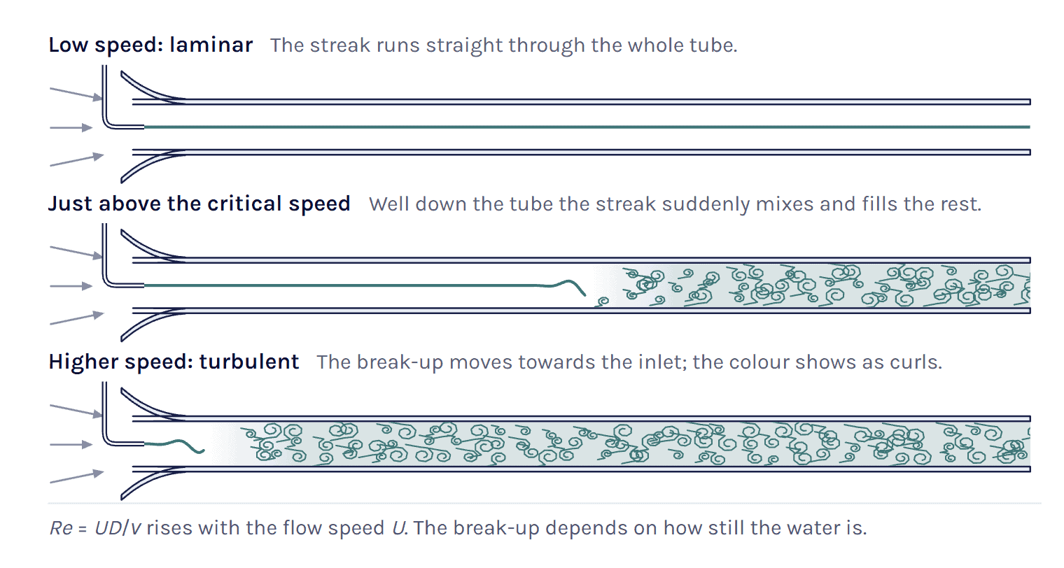
Reynolds’ colour-band experiment. At a low speed the dye streak runs straight through the tube (laminar). Just above the critical speed it suddenly breaks up some way down the tube (transition), and at higher speeds the break-up moves closer to the inlet (turbulent). Own drawing after Reynolds (1883) [14]. The figure as an image (PNG).

He also found that the speed at which the eddies appeared was inversely proportional to the tube diameter and fell as the water got warmer [14], in other words as its viscosity dropped. Both point to UD/ν, the ratio now called the Reynolds number [12]. The critical speed was also very sensitive to disturbances in the water before it entered the tubes [14]. So there is no one Reynolds number where every pipe flow turns turbulent. It depends on how disturbed the water is.

The calculator’s small-tube example shows the laminar case of Reynolds’ experiment, a straight dye thread, for water at 20 °C in a 4 mm tube at 0.3 m/s (Re ≈ 1200).

Flow regimes by geometry

The table gives the regimes for the four shapes in the calculator. Read the pipe rows with Re on D or D_h, the plate rows with Re_x, and the cylinder and sphere rows with Re on the diameter. Where the sources spread, the second line in the first column says how far.

Flow regimes by geometry. Each shape has its own Reynolds number and its own length. The limits are approximate: the second line in the first column gives the zone where the sources spread, and no limit is a sharp line.

Pipe or duct Re on the inner diameter D, or on D_h for a duct

Flow regimes: Pipe or duct (Re on the inner diameter D, or on Dh for a duct)
Reynolds number	Regime	What the flow does (sources)	In the calculator
below 2300edge between 2000 and 2300	Laminar	Fully turbulent flow cannot sustain itself below about 2300. A disturbance makes at most local puffs, and below about 2040 even those die out. [10], [11], [12], [13]	Use ↑
2300 to about 4000edge between 3000 and 4000	Transitional	Laminar or turbulent, depending on the inlet and on disturbances. Turbulent patches come and go, so treat friction and heat transfer as uncertain. [10], [12], [13]	Use ↑
above about 4000	Turbulent	Turbulent in ordinary pipes. Laminar flow survives here only with an exceptionally quiet inlet (Reynolds kept it to about 13 000). [12], [13]	Use ↑

Flat plate, no pressure gradient Re_x on the distance x from the leading edge

Flow regimes: Flat plate, no pressure gradient (Rex on the distance x from the leading edge)
Reynolds number	Regime	What the flow does (sources)	In the calculator
below 5 × 10⁵	Laminar boundary layer	Below the engineering critical value the boundary layer is most likely laminar. A turbulent free stream can start transition earlier. [15], [16]	Use ↑
5 × 10⁵ to 3.9 × 10⁶edge between 2.8 × 10⁶ and 3.9 × 10⁶	Transition possible	Past the engineering value transition can start. Where depends on how quiet the free stream is, and in a very quiet tunnel it began near 2.8 × 10⁶. [15], [16]	Use ↑
above 3.9 × 10⁶	Turbulent boundary layer	Turbulent. Even at the lowest turbulence Schubauer and Skramstad reached (below about 0.1 %), transition was complete by about 3.9 × 10⁶. [16]	Use ↑

Circular cylinder in cross flow Re on the diameter

Flow regimes: Circular cylinder in cross flow (Re on the diameter)
Reynolds number	Regime	What the flow does (sources)	In the calculator
below 6.29	Attached flow	The flow follows the surface all round, with no separation. [17]	Use ↑
6.29 to 40edge between 40 and 50	Steady separated wake	Two fixed, symmetric eddies sit behind the cylinder, and nothing is shed. [17], [18]	Use ↑
40 to 188.5edge between 150 and 188.5	Laminar vortex street	Vortices are shed alternately and regularly from each side, a two-dimensional Kármán vortex street. [18], [19]	Use ↑
188.5 to 300edge between 259 and 300	Wake transition	The street becomes three-dimensional (instability modes appear at 188.5 and 259), and turbulence starts in the free shear layers that leave the cylinder. [18], [19]	Use ↑
300 to about 2 × 10⁵	Subcritical	The boundary layer separates while still laminar. The wake is turbulent and vortex shedding continues. [18], [20]	Use ↑
about 2 × 10⁵ to 10⁶edge between 5.5 × 10⁵ and 10⁶	Critical (drag crisis)	The laminar boundary layer separates, turns turbulent and reattaches (a separation bubble), so the flow stays attached further round and the drag drops. Regular shedding was still seen at 5.5 × 10⁵. [20], [21], [22]	Use ↑
10⁶ to 3.5 × 10⁶edge between 3.5 × 10⁶ and 5 × 10⁶	Supercritical	The boundary layer turns turbulent ahead of separation, and the drag is low. It then rises again towards 3.5 × 10⁶. [20], [21], [23]	Use ↑
above 3.5 × 10⁶	Transcritical	The drag settles at about 0.7 and regular vortex shedding returns (Strouhal number about 0.25 to 0.29). The sources put the start between 3.5 × 10⁶ and about 5 × 10⁶. [21], [23], [24]	Use ↑

Sphere Re on the diameter

Flow regimes: Sphere (Re on the diameter)
Reynolds number	Regime	What the flow does (sources)	In the calculator
below 1	Stokes (creeping) flow	Viscous forces dominate. For Re much less than 1 inertia is negligible and the Stokes equations apply. [25]	Use ↑
1 to 20.5	Attached, steady	Inertia matters, but the flow still follows the whole surface and has not separated yet. [26]	Use ↑
20.5 to 210edge between 200 and 210	Steady axisymmetric wake	A steady ring vortex sits behind the sphere. [26], [27], [28]	Use ↑
210 to 270edge between 270 and 300	Steady non-axisymmetric wake	The wake loses its symmetry but is still steady. [27], [28]	Use ↑
270 to 6000edge between 3000 and 6000	Periodic shedding	Hairpin vortices are shed periodically, and the wake is unsteady. [27], [29]	Use ↑
6000 to 3.7 × 10⁵edge between 3 × 10⁵ and 3.8 × 10⁵	Subcritical	The wake fluctuates strongly and periodically, up to the drag crisis. [29], [30]	Use ↑
above 3.7 × 10⁵	Past the drag crisis	Above about 3.7 × 10⁵ Achenbach no longer detected periodic shedding, and the wake forms a pair of streamwise vortices (observed to 10⁶). [29], [30], [31]	Use ↑

For a duct, the pipe limits on D_h are a guide, not exact values.

For the cylinder and the sphere the critical range is for smooth bodies in wind tunnels, and roughness moves it. Achenbach’s spheres were measured at about 0.45 % turbulence.

The regime map: the four shapes on one logarithmic Re axis, drawn from the same data as the calculator and the table. Blended, hatched zones mark edges that are not sharp, where the sources differ or around an edge that one source gives as a single value. The marks above the axis are everyday flows for scale, our own arithmetic for stated cases and a measured value for the aorta [32]. The map in the calculator also shows swimming microorganisms [33]. Own illustration. The figure as an image (PNG).

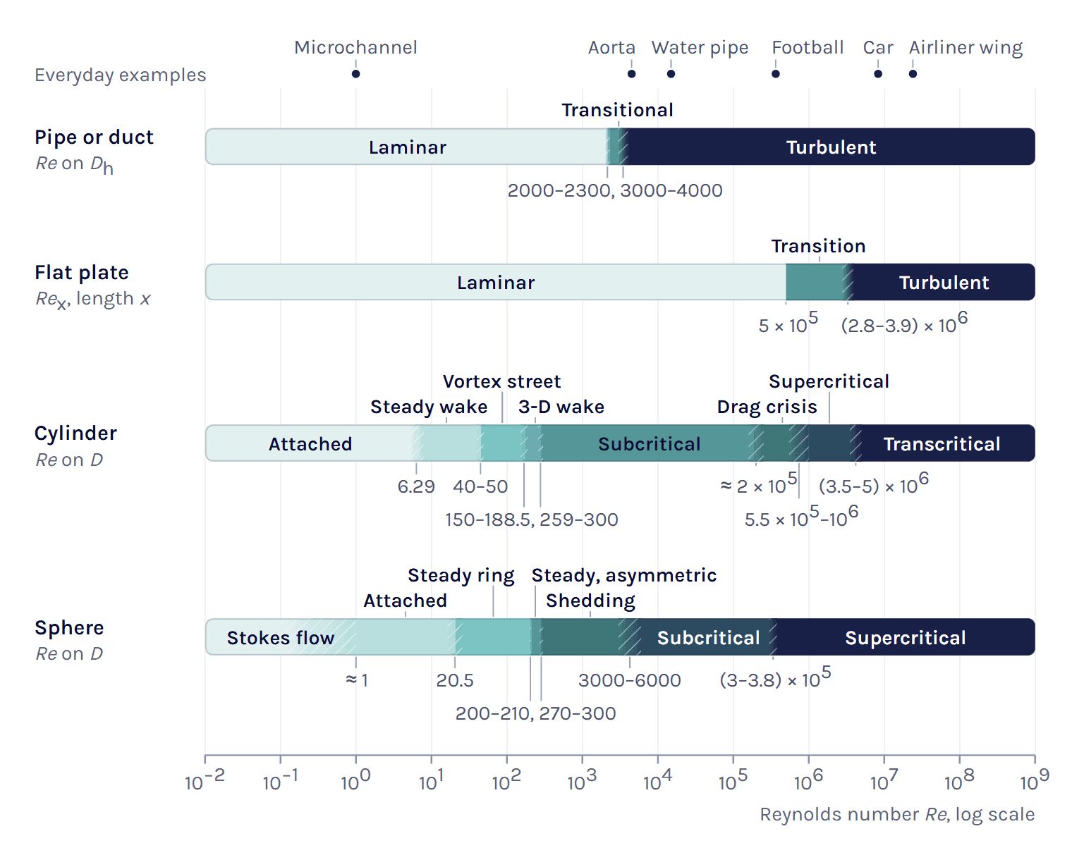
The same number means different things for different shapes. At Re = 5 × 10⁵ a pipe flow is far into the turbulent range, while on a flat plate this is the engineering critical value of Re_x, where the boundary layer goes from most likely laminar to most likely turbulent [15]. A smooth cylinder is past its critical Reynolds number of about 2 × 10⁵ [18], and a smooth sphere is past the 3.7 × 10⁵ that Achenbach measured [29].

Critical Reynolds number

Reynolds also found a second, lower critical speed in a pipe, at which eddies that are already there die out along the pipe [14], and the critical value he estimated is about 2000 [10]. Avila et al. later pinned down where turbulence becomes sustained, at Re = 2040 ± 10. Below it a turbulent puff is more likely to decay than to split, and above it the puffs split and spread [10, 11]. Mukund and Hof put the critical point between 2020 and 2060, and between about 1700 and 2300 they found turbulence only as such local puffs, with fully turbulent flow collapsing into them [12].

Above that, the Reynolds number alone does not decide. Reynolds found that with enough care in setting up the pipe, turbulence could be put off to about 13 000 [12], and laminar pipe flow is linearly stable to at least Re = 10⁷ [10]. Without that care it turns turbulent much earlier. Even in Mukund and Hof’s 4 mm research pipe natural transition came at about 3000 [12], and a university physics textbook gives turbulent flow above about 3000 [13]. The calculator draws its transitional band from 2300 to about 4000, a round upper limit with some margin above 3000. Treat that band as a warning in a real system with bends and valves upstream, where both kinds of flow are possible.

On a flat plate with no pressure gradient, the engineering critical value is Re_x,cr = 5 × 10⁵ [15]. Where transition really starts depends on how quiet the free stream is. Schubauer and Skramstad brought the turbulence in their wind tunnel below about 0.1 %, and transition then began at Re_x ≈ 2.8 × 10⁶ and ended at about 3.9 × 10⁶. At 0.34 % it began near 1.5 × 10⁶ [16]. More turbulence in the free stream brings it earlier still. The calculator therefore draws the plate band from 5 × 10⁵ to 3.9 × 10⁶.

Critical means something else for a cylinder or a sphere, where it marks the drag crisis. On a cylinder the laminar boundary layer separates, turns turbulent and reattaches, so the final separation moves aft and the drag drops [20, 21]. Roshko gives about 2 × 10⁵ for the cylinder [18], and for a smooth sphere Achenbach found an upper critical value of 3.7 × 10⁵, above which he could no longer detect periodic shedding [29]. Neither is a fixed number. Achenbach’s drag measurements on spheres were made at about 0.45 % free-stream turbulence [31], and roughness moves the crisis to a lower Reynolds number, as the drag coefficient calculator page shows for golf balls.

Pipes and ducts

Hydraulic diameter

For a duct that is not round, Re uses the hydraulic diameter, with A the cross-section area and P the wetted perimeter, the length of wall in contact with the fluid.

D_h = 4A / P (2)

A round pipe gives D_h = D, and a rectangle a × b gives 2ab/(a + b). A concentric annulus gives D_o − D_i and two wide parallel plates with a gap h give 2h. The free surface of a part-full pipe or an open channel is not wetted, so it stays out of P. Note that hydraulics texts often use the hydraulic radius R_h = A/P = D_h/4 instead, and a Reynolds number on R_h is 4 times smaller for the same flow.

D_h = 4A/P, with A the flow area (hatched) and P the wetted perimeter (thick teal line).

Circular pipe

A = πD²/4

P = πD

D_h = D

The pipe diameter itself.

Rectangular duct

A = ab

P = 2(a + b)

D_h = 2ab/(a + b)

A square duct gives D_h = a.

Annulus

A = π(D_o² − D_i²)/4

P = π(D_o + D_i)

D_h = D_o − D_i

Both walls count in P.

Parallel plates

A = hW

P ≈ 2W

D_h = 2h

Some texts use h instead; say which.

Example: a 200 × 100 mm duct has D_h = 133 mm. Take the velocity from the real area, U = Q/A. Dividing Q by πD_h²/4 instead gives a speed 43 % too high.

Hydraulic diameter D_h = 4A/P for a circle, a rectangle, an annulus and two parallel plates. Only the wetted wall counts in P. Own illustration.

The hydraulic diameter is a convenient length, not an exact equivalence. Fully developed laminar flow in a round pipe has a Darcy friction factor f = 64/Re [10], but with D_h the exact laminar solution gives f·Re = 56.9 for a square duct and 96 between parallel plates (our calculation), about 11 % below and 50 % above 64/Re.

Reynolds number from a flow rate

When you know the flow rate rather than the speed, the mean speed is U = Q/A for a volume flow Q, or U = ṁ/(ρA) for a mass flow ṁ, and Re follows from (1). For a round pipe the area drops out.

Re = 4ṁ / (πDμ) = 4Q / (πDν) (3)

The mass-flow form needs only μ, not the density. Take the same 25 mm water pipe at 0.5 kg/s. Then Re = 4 × 0.5 / (π × 0.025 × 1.0016 × 10⁻³) = 2.54 × 10⁴, and the mean speed is 0.5 / (998.2 × 4.909 × 10⁻⁴) = 1.02 m/s. For a duct of any other shape, use the real cross-section area for A and D_h only as the length. The HVAC example below shows what goes wrong otherwise.

Development length near an inlet

Close to an inlet the flow has not settled yet. Durst et al. give the laminar development length of a round pipe, the distance to the parabolic profile, as L/D ≈ 0.0567 Re at large Re [34], and the 4 mm tube at Re ≈ 1200 then needs about 68 diameters, 0.27 m. Turbulent flow has no such simple rule. At Re = 3.9 × 10⁵, Barbin and Jones found the wall shear stress developed within 15 diameters, but the velocity profile was still developing after 40 [35].

Flat plate and the transition point

Along a flat plate the boundary layer starts laminar at the leading edge and grows with the distance x, and so does the local Reynolds number Re_x = Ux/ν [15]. With the engineering critical value of 5 × 10⁵, transition is expected to start at

x_cr = Re_x,cr ν / U (4)

In air at 20 °C and 20 m/s this gives x_cr = 5 × 10⁵ × 1.506 × 10⁻⁵ / 20 = 0.38 m. The 3.5 m plate of the example has Re_L = 4.65 × 10⁶, and transition is expected from about 0.38 m, so roughly the first 11 % of the plate is laminar. A very quiet stream could delay it to Re_x ≈ 2.8 × 10⁶, 2.1 m from the leading edge, with the layer turbulent by about 2.9 m [16], and a turbulent free stream brings it forward.

Load the plate example in the calculator ↑

A flat-plate boundary layer in air at 20 °C and 20 m/s, drawn to scale along a 3.5 m plate: laminar from the leading edge, transition from x_cr = 0.38 m, or from 2.1 to 2.9 m in a very quiet stream, then turbulent [16]. The thickness, exaggerated by the factor given in the figure, follows the laminar (Blasius) and turbulent power-law estimates of Schlichting [36]. Own illustration.

The same numbers tell you whether a CFD model of the plate can be fully turbulent from the leading edge or whether a transition model is worth the extra cost (see the Simcenter STAR-CCM+ section).

Cylinder and sphere

Behind a circular cylinder the wake changes several times as Re rises. Sen et al. computed that the flow first separates at Re = 6.29 [17], and up to about 40 two steady eddies sit behind the cylinder. Roshko measured regular vortex streets from about 40 to 150, a transition range from 150 to 300 and an irregular range above 300, where turbulence comes with the shedding [18]. Barkley and Henderson found that the two-dimensional street turns three-dimensional at Re = 188.5 [19], and a 2D simulation cannot follow that.

Periodic shedding has been seen up to about 2 × 10⁵ [18], and Bearman still found narrow-band shedding at 5.5 × 10⁵, well into the critical range [22]. Achenbach describes the drag crisis in three states, from laminar separation (subcritical) through a separation bubble with turbulent reattachment (critical) to a boundary layer that turns turbulent before it separates (supercritical) [20]. Above 3.5 × 10⁶ Roshko found the drag coefficient back at 0.7 and regular shedding again [23], and Schewe puts the start of this transcritical range at about 5 × 10⁶ [21].

Attached

Re below 6.29

The flow follows the surface all round.

Twin eddies

Re 6.29 to 40–50

Two fixed eddies sit behind it; nothing is shed.

Vortex street

Re 40–50 to 150–188.5

Vortices shed alternately from each side.

Turbulent wake

Re 150–188.5 to ≈ 2 × 10⁵

The wake turns 3-D, then turbulent; laminar separation, wide wake.

Supercritical

Re 5.5 × 10⁵–10⁶ to (3.5–5) × 10⁶

Turbulent boundary layer, later separation, narrow wake.

Between the last two lies the drag crisis, Re ≈ 2 × 10⁵ to 5.5 × 10⁵–10⁶: the laminar boundary layer separates, turns turbulent and reattaches, so the final separation moves aft and the drag drops. Above (3.5–5) × 10⁶ (transcritical) regular shedding returns.

The wake of a circular cylinder by Reynolds number, from attached flow to the transcritical range, with the band edges of the calculator. Schematic, not a simulation. Own drawing.

The shedding frequency follows from the Strouhal number, St = fD/U, and Roshko found St essentially constant, at about 0.21, in the irregular range that he measured up to Re = 10⁴ [18].

Strouhal number of a cylinder by Reynolds number

Roshko fitted St = 0.212(1 − 21.2/Re) for Re from 50 to 150 and 0.212(1 − 12.7/Re) from 300 to 2000 [18]. The sources used here give no single value between 10⁴ and the transcritical range, and the calculator shows no frequency there. In the drag crisis Bearman measured Strouhal numbers up to 0.46 [22]. In the transcritical range, which starts between 3.5 × 10⁶ and about 5 × 10⁶, Roshko measured 0.27 [23], Achenbach and Heinecke 0.25 ± 0.018 [24] and Schewe 0.29 at 7.1 × 10⁶ [21].

Dennis and Walker computed that flow past a sphere first separates at Re = 20.5 [26]. Johnson and Patel found a steady, axisymmetric wake up to Re = 200, a steady but non-axisymmetric wake from 210 to 270 and periodic shedding above 270 [27]. Achenbach saw strong periodic fluctuations in the wake from 6000 to 3 × 10⁵ and could no longer detect periodic shedding above 3.7 × 10⁵ [29], and Taneda saw the wake form a pair of streamwise vortices from 3.8 × 10⁵ [30].

The calculator’s football example, a 0.22 m ball at 25 m/s in air at 20 °C, has Re = 3.65 × 10⁵, just below that edge and inside the zone where these sources put the crisis. For the drag coefficient itself, use the drag coefficient calculator.

Worked examples

HVAC duct: hydraulic diameter and flow rate

A rectangular ventilation duct of 400 × 200 mm carries air at 20 °C and 1 atm at a mean speed of 5 m/s. The hydraulic diameter is D_h = 2 × 0.4 × 0.2 / (0.4 + 0.2) = 0.267 m, and Re = 5 × 0.267 / (1.506 × 10⁻⁵) = 8.85 × 10⁴. The flow is turbulent. Taking the width of 400 mm as the length would give 1.33 × 10⁵, 50 % too high.

The volume flow is Q = UA = 5 × 0.08 = 0.4 m³/s, or 1440 m³/h. If you start from that flow rate, divide it by the real area of 0.08 m². Dividing by the area of a circle with diameter D_h, π × 0.267²/4 = 0.0559 m², gives 7.16 m/s, 43 % too high, and Re comes out at 1.27 × 10⁵.

Load the duct example in the calculator ↑

Cable in wind: vortex shedding

A 20 mm cable in a 5 m/s wind at 20 °C has Re = 5 × 0.02 / (1.506 × 10⁻⁵) = 6640. That is in the subcritical range, where the wake is turbulent and still sheds vortices, and inside the range where Roshko found St ≈ 0.21 [18]. The shedding frequency is f = St·U/D ≈ 0.21 × 5 / 0.02 = 52.5 Hz, the number you compare with the natural frequencies of the cable and its supports. A laminar vortex street, Re from about 40 to 150, would need the wind to drop to 0.03 to 0.11 m/s.

Load the cable example in the calculator ↑

Model in a wind tunnel: matching the Reynolds number

Two geometrically similar flows with the same Reynolds number have the same balance between inertial and viscous forces [1], and that is why you test a scale model at the full-scale Re where you can. Take a car of 4.5 m at 100 km/h in air at 20 °C (example values, not a particular car). Its Reynolds number is Re = 27.8 × 4.5 / (1.506 × 10⁻⁵) = 8.30 × 10⁶, and a 1:4 model, 1.125 m long, needs four times the speed, 111 m/s or 400 km/h.

That is Mach 0.32, with a speed of sound of a = √(γRT) = 343 m/s at 20 °C and γ = 1.4 [37, 38]. The density at the nose is then about 5 % above the free stream in isentropic flow [37], and the model no longer matches the car on Mach number. Water at 20 °C, with a kinematic viscosity 15 times lower, lets the same model run at 7.40 m/s. The Match this Re button in the calculator does this in one step and warns about the Mach number.

Load the wind-tunnel example in the calculator ↑

Reynolds number in Simcenter STAR-CCM+

In Simcenter STAR-CCM+ the Reynolds number is the first thing to check before you choose the physics models, since the Viscous Regime group asks you to pick Inviscid, Laminar or Turbulent [39]. The S-bend tutorial in the documentation runs the same 2 cm pipe twice, laminar at Re = 500 and turbulent at Re = 50 000 [39]. Its material has a constant density of 1 kg/m³ and a dynamic viscosity of 1.716 × 10⁻⁵ Pa·s, and with an inlet velocity of 0.429 m/s that gives Re = 1 × 0.429 × 0.02 / (1.716 × 10⁻⁵) = 500.

Note that the density of 1 kg/m³ is a value chosen for the tutorial, not air. Real air at 20 °C at the same speed gives Re = 570, laminar as well. For Re = 50 000 the tutorial raises the speed to 42.9 m/s, and the turbulent part uses the Realizable K-Epsilon Two-Layer model with the Two-Layer All y+ Wall Treatment [39].

When Re falls in the transitional range of a pipe, we run the case both laminar and turbulent and compare, and treat the difference as part of the uncertainty.

From the Reynolds number to the Simcenter STAR-CCM+ settings: the Viscous Regime, the Equation of State and the Material Properties for Density and Dynamic Viscosity. Own drawing of the model names in the documentation [39], not a screenshot.

Material properties

The fluid models in the calculator have counterparts with the same names in Simcenter STAR-CCM+. The equation of state models include Constant Density, Ideal Gas and IAPWS-IF97 (Water), and the Dynamic Viscosity methods include Constant and Sutherland’s Law. All of them except Constant Density and Constant need an Energy model in the continuum, and IAPWS-IF97 (Water) also needs a liquid material [39]. Sutherland’s Law has the same form as the law in the calculator. The calculator’s Simcenter STAR-CCM+ panel gives you Density and Dynamic Viscosity in kg/m^3 and Pa-s to copy for a constant-property case. If your properties depend on temperature, the documentation suggests checking that numbers such as Re and the Prandtl number keep the values you expect [39].

At very low pressure the calculator also checks the Knudsen number for air, Kn = (Ma/Re)√(γπ/2), the form the documentation gives for high Reynolds numbers. The documentation treats the flow as a continuum only below Kn = 0.01 [39].

Local Reynolds number as a field function

The field function library has Reynolds numbers for particles and phase pairs in multiphase models, and some that belong to turbulence and transition models, but none for the bulk flow [39]. So we write Re as a user field function. With the Density and DynamicViscosity field functions and a length typed in metres, here the 25 mm pipe, a local Re based on the speed in each cell is

$Density * mag($$Velocity) * 0.025 / $DynamicViscosity

This is our construction from the documented syntax, where $ marks a scalar and $$ a vector field function [39]. Replace 0.025 with your own length.

Transition models

If your Re puts a boundary layer in a transition band, a flat plate past Re_x = 5 × 10⁵ for example, a transition model predicts where it turns turbulent instead of assuming it is turbulent everywhere. Gamma ReTheta and Gamma work with SST (Menter) K-Omega, and SA Gamma with Standard Spalart-Allmaras [39]. The transition guidelines ask for a wall y+ between 0.1 and 1 and, for natural and low free-stream bypass transition, a free-stream turbulent viscosity ratio between 1 and 10 [39]. You can size the first cell with the y+ calculator and the inlet with the turbulence boundary conditions calculator. Our blog post Transition modelling in Simcenter STAR-CCM+ collects more on these models.

If you are not sure which of laminar, turbulent or a transition model your case needs, the turbulence model selector is one place to start. You can also use the form below and choose Technical question.

References and changelog

References

[1] NASA Glenn Research Center, Reynolds number, Beginner’s Guide to Aeronautics. https://www.grc.nasa.gov/www/k-12/airplane/reynolds.html

[2] A. Thompson and B. N. Taylor, Guide for the Use of the International System of Units (SI), NIST Special Publication 811, 2008 edition, Appendix B.8.

[3] IAPWS R12-08, Release on the IAPWS Formulation 2008 for the Viscosity of Ordinary Water Substance, 2008.

[4] IAPWS R7-97(2012), Revised Release on the IAPWS Industrial Formulation 1997 for the Thermodynamic Properties of Water and Steam.

[5] E. W. Lemmon, R. T Jacobsen, S. G. Penoncello and D. G. Friend, Thermodynamic properties of air and mixtures of nitrogen, argon, and oxygen from 60 to 2000 K at pressures to 2000 MPa, Journal of Physical and Chemical Reference Data 29(3), 331–385, 2000.

[6] U.S. Standard Atmosphere, 1976, NOAA, NASA and USAF, NASA-TM-X-74335 (Sutherland constant S = 110.4 K).

[7] E. W. Lemmon and R. T Jacobsen, Viscosity and thermal conductivity equations for nitrogen, oxygen, argon, and air, International Journal of Thermophysics 25(1), 21–69, 2004.

[8] Y. A. Çengel and J. M. Cimbala, Fluid Mechanics: Fundamentals and Applications, 3rd ed., McGraw-Hill, 2014, Tables A-3 and A-9.

[9] ITTC Recommended Procedures and Guidelines 7.5-02-01-03, Fresh water and seawater properties, International Towing Tank Conference, 2011.

[10] D. Barkley, Theoretical perspective on the route to turbulence in a pipe, Journal of Fluid Mechanics 803, P1, 2016. https://doi.org/10.1017/jfm.2016.465

[11] K. Avila, D. Moxey, A. de Lozar, M. Avila, D. Barkley and B. Hof, The onset of turbulence in pipe flow, Science 333, 192–196, 2011. https://doi.org/10.1126/science.1203223

[12] V. Mukund and B. Hof, The critical point of the transition to turbulence in pipe flow, Journal of Fluid Mechanics 839, 76–94, 2018. https://doi.org/10.1017/jfm.2018.31

[13] W. Moebs, S. J. Ling and J. Sanny, University Physics Volume 1, OpenStax, Rice University, 2016, section 14.7 Viscosity and turbulence. https://openstax.org/books/university-physics-volume-1/pages/14-7-viscosity-and-turbulence

[14] O. Reynolds, An experimental investigation of the circumstances which determine whether the motion of water shall be direct or sinuous, and of the law of resistance in parallel channels, Philosophical Transactions of the Royal Society of London 174, 935–982, 1883. https://doi.org/10.1098/rstl.1883.0029

[15] J. M. Cimbala, Turbulent flat plate boundary layer, ME 320 lesson notes 13D, Penn State University (figures and tables from Y. A. Çengel and J. M. Cimbala, Fluid Mechanics, 4th ed.). https://me.psu.edu/cimbala/me320/Lesson_Notes/Fluid_Mechanics_Lesson_13D.pdf

[16] G. B. Schubauer and H. K. Skramstad, Laminar-boundary-layer oscillations and transition on a flat plate, NACA Report 909, 1948 (also Journal of Research of the National Bureau of Standards 38, 251–292, 1947), figure 7. https://ntrs.nasa.gov/citations/19930091976

[17] S. Sen, S. Mittal and G. Biswas, Steady separated flow past a circular cylinder at low Reynolds numbers, Journal of Fluid Mechanics 620, 89–119, 2009. https://doi.org/10.1017/S0022112008004904

[18] A. Roshko, On the development of turbulent wakes from vortex streets, NACA Report 1191, 1954. https://ntrs.nasa.gov/citations/19930092207

[19] D. Barkley and R. D. Henderson, Three-dimensional Floquet stability analysis of the wake of a circular cylinder, Journal of Fluid Mechanics 322, 215–241, 1996. https://doi.org/10.1017/S0022112096002777

[20] E. Achenbach, Distribution of local pressure and skin friction around a circular cylinder in cross-flow up to Re = 5 × 10⁶, Journal of Fluid Mechanics 34, 625–639, 1968. https://doi.org/10.1017/S0022112068002120

[21] G. Schewe, On the force fluctuations acting on a circular cylinder in crossflow from subcritical up to transcritical Reynolds numbers, Journal of Fluid Mechanics 133, 265–285, 1983. https://doi.org/10.1017/S0022112083001913

[22] P. W. Bearman, On vortex shedding from a circular cylinder in the critical Reynolds number régime, Journal of Fluid Mechanics 37, 577–585, 1969. https://doi.org/10.1017/S0022112069000735

[23] A. Roshko, Experiments on the flow past a circular cylinder at very high Reynolds number, Journal of Fluid Mechanics 10, 345–356, 1961. https://doi.org/10.1017/S0022112061000950

[24] E. Achenbach and E. Heinecke, On vortex shedding from smooth and rough cylinders in the range of Reynolds numbers 6 × 10³ to 5 × 10⁶, Journal of Fluid Mechanics 109, 239–251, 1981. https://doi.org/10.1017/S002211208100102X

[25] I. Proudman and J. R. A. Pearson, Expansions at small Reynolds numbers for the flow past a sphere and a circular cylinder, Journal of Fluid Mechanics 2, 237–262, 1957. https://doi.org/10.1017/S0022112057000105

[26] S. C. R. Dennis and J. D. A. Walker, Calculation of the steady flow past a sphere at low and moderate Reynolds numbers, Journal of Fluid Mechanics 48, 771–789, 1971. https://doi.org/10.1017/S0022112071001848

[27] T. A. Johnson and V. C. Patel, Flow past a sphere up to a Reynolds number of 300, Journal of Fluid Mechanics 378, 19–70, 1999. https://doi.org/10.1017/S0022112098003206

[28] R. Natarajan and A. Acrivos, The instability of the steady flow past spheres and disks, Journal of Fluid Mechanics 254, 323–344, 1993. https://doi.org/10.1017/S0022112093002150

[29] E. Achenbach, Vortex shedding from spheres, Journal of Fluid Mechanics 62, 209–221, 1974. https://doi.org/10.1017/S0022112074000644

[30] S. Taneda, Visual observations of the flow past a sphere at Reynolds numbers between 10⁴ and 10⁶, Journal of Fluid Mechanics 85, 187–192, 1978. https://doi.org/10.1017/S0022112078000580

[31] E. Achenbach, Experiments on the flow past spheres at very high Reynolds numbers, Journal of Fluid Mechanics 54, 565–575, 1972. https://doi.org/10.1017/S0022112072000874

[32] A. F. Stalder, A. Frydrychowicz, M. F. Russe, J. G. Korvink, J. Hennig, K. Li and M. Markl, Assessment of flow instabilities in the healthy aorta using flow-sensitive MRI, Journal of Magnetic Resonance Imaging 33, 839–846, 2011. https://doi.org/10.1002/jmri.22512

[33] E. Lauga and T. R. Powers, The hydrodynamics of swimming microorganisms, Reports on Progress in Physics 72, 096601, 2009. https://doi.org/10.1088/0034-4885/72/9/096601

[34] F. Durst, S. Ray, B. Ünsal and O. A. Bayoumi, The development lengths of laminar pipe and channel flows, Journal of Fluids Engineering 127, 1154–1160, 2005. https://doi.org/10.1115/1.2063088

[35] A. R. Barbin and J. B. Jones, Turbulent flow in the inlet region of a smooth pipe, Journal of Basic Engineering 85, 29–33, 1963. https://doi.org/10.1115/1.3656521

[36] H. Schlichting, Lecture series “Boundary layer theory”, Part I Laminar flows and Part II Turbulent flows, NACA TM 1217 and TM 1218, 1949. https://ntrs.nasa.gov/citations/20040021320

[37] Ames Research Staff, Equations, tables, and charts for compressible flow, NACA Report 1135, 1953, equation 45.

[38] NASA Glenn Research Center, Isentropic flow equations, Beginner’s Guide to Aeronautics. https://www.grc.nasa.gov/www/k-12/airplane/isentrop.html

[39] Simcenter STAR-CCM+ documentation, version 2606, Siemens Digital Industries Software, 2026 (tutorial Laminar and Turbulent Flow in an S-Bend, the Viscous Regime, Equation of State and Gamma transition model references, the Field Function Library, User Field Function Examples, Transition Guidelines, Flow Regimes, and Guidelines for Fluid Flow and Energy).

Changelog

October 2026: first published, with the calculator, the regime map and this guide. The fluid properties and regime limits were checked against the sources listed above, apart from the two band edges given as “about” in the table.

Questions about the Reynolds number

Ask a Volupe specialist

Christoffer Johansson

Senior Application Specialist, M.Sc.

Questions about laminar, turbulent or transition set-ups? We reply within one day.

Ask a technical question →

At what Reynolds number is flow laminar or turbulent?

It depends on the shape. Pipe flow is laminar below about 2000 and turbulent above about 3000, with either possible in between, and the calculator draws its transitional band from 2300 to 4000. On a flat plate the engineering value is Reₓ = 5 × 10⁵, though transition can wait until about 2.8 × 10⁶ in a very quiet stream. A cylinder or a sphere has no single value. Its wake changes step by step, up to the drag crisis at about 2 × 10⁵ for a cylinder and 3.7 × 10⁵ for a smooth sphere.

What does a Reynolds number of 500,000 mean?

It depends on the shape the number belongs to. Pipe flow at Re = 5 × 10⁵ is far into the turbulent range. On a flat plate the same number is the engineering critical value of the local Reynolds number Reₓ, below which the boundary layer is most likely laminar and above which it is most likely turbulent. A smooth cylinder is past its critical Reynolds number of about 2 × 10⁵, in the drag crisis, and a smooth sphere is past the upper critical value of 3.7 × 10⁵ that Achenbach measured.

What if the Reynolds number is between 2000 and 3000?

That is the range where pipe flow can be either. Below about 2000 turbulence dies out on its own, and Avila et al. put the point where it becomes sustained at Re = 2040 ± 10. Up to about 2300 turbulence comes only as local puffs that travel with the flow, and above that it can spread. Whether a given pipe is then laminar or turbulent depends on how disturbed the inlet is, and in a carefully built rig Mukund and Hof saw natural transition at about 3000. In CFD we run such a case both laminar and turbulent and compare.

What is the critical Reynolds number for a flat plate?

The engineering value is Reₓ = 5 × 10⁵, with x measured from the leading edge. Below it the boundary layer is most likely laminar and above it most likely turbulent. Transition is then expected from x = 5 × 10⁵ ν/U, 0.38 m in air at 20 °C and 20 m/s. Where it really starts depends on how quiet the free stream is. In a wind tunnel with less than about 0.1 % turbulence, Schubauer and Skramstad saw transition begin only at about 2.8 × 10⁶.

How do I find the Reynolds number from a mass flow rate?

Divide the mass flow by the density and the cross-section area to get the mean speed, U = ṁ/(ρA), and use it in Re = ρUD/μ. In a round pipe this becomes Re = 4ṁ/(πDμ), which needs only the dynamic viscosity. Water at 20 °C flowing at 0.5 kg/s in a 25 mm pipe gives Re = 4 × 0.5/(π × 0.025 × 1.0016 × 10⁻³) = 2.54 × 10⁴. For a duct of another shape, use Re = ṁDₕ/(Aμ), with the real area A and the hydraulic diameter Dₕ.

Does the Reynolds number have units?

No. In Re = ρUL/μ the numerator has the units kg/m³ × m/s × m and the denominator Pa·s, which is kg/(m·s), so the units cancel and leave a pure number. The value is the same in SI and US units as long as every input is converted consistently, for example with the kinematic viscosity in m²/s and not in cSt.

What is the difference between dynamic and kinematic viscosity?

The dynamic viscosity μ (Pa·s, or cP = mPa·s) relates the shear stress in the fluid to the velocity gradient. The kinematic viscosity ν (m²/s, or cSt = mm²/s) is the dynamic viscosity divided by the density, ν = μ/ρ. Water at 20 °C has μ = 1.002 mPa·s and ν = 1.003 mm²/s. Air at 20 °C has a dynamic viscosity 55 times lower than water but a kinematic viscosity 15 times higher, and at the same speed and size you get a Reynolds number 15 times lower in air.

Which length should I use in the Reynolds number?

The one the regime limits you compare with are based on. That is the inner diameter for a round pipe, the hydraulic diameter Dₕ = 4A/P for any other duct, the distance from the leading edge for a flat plate, and the diameter for a cylinder or a sphere. Hydraulics texts sometimes use the hydraulic radius, a quarter of Dₕ, which gives a Reynolds number 4 times smaller.

Can Volupe help me choose laminar, turbulent or transition physics in Simcenter STAR-CCM+?

Yes. Our application engineers help Simcenter STAR-CCM+ users with set-ups like these, from the material properties and the Viscous Regime to transition models and the mesh near the wall. Customers with maintenance get this through our support, and we also run Simcenter STAR-CCM+ training courses.

Talk to an engineer in your region

Every Volupe business developer holds an engineering degree. Find your regional contact below, or send us a message.

Send a message See all sales regions

Denmark and Central Eastern Europe

Lukas Johansson

Sales Director, M.Sc.

+46 70 446 62 97 LinkedIn

Norway, Finland and the Baltics

Carl Wanngård

Business Developer, M.Sc.

+46 73 147 33 20 LinkedIn

DACH region

David Fabis

Business Developer, M.Sc.

+49 151 2103 4599 LinkedIn

DACH region

André Hau

Business Developer, M.Sc.

+49 175 522 3159 Email

Sweden

Fredrik Liljedahl

Business Developer, M.Sc.

+46 76 447 99 45 LinkedIn

Europe

Henrik Pahlitzsch

Business Developer, M.Sc.

+46 76 870 11 40

Iberia

Mikel Sevilla

Business Developer

+34 636 421 923 LinkedIn

Ask us about Reynolds number calculator

Use this form for licence quotes, demos, training and technical questions.

What happens next

A reply within one day.
A scoping call with one of our engineers.
A quote, demo or other next step that fits your enquiry.

After purchase: support from Volupe simulation engineers.

Reynolds number calculator

Reynolds number and flow regime calculator

Size

Flow

Fluid

Reynolds number

Simcenter STAR-CCM+ settings

Regime map

Reynolds number formula

Which length to use

Dynamic and kinematic viscosity

How to calculate the Reynolds number

Laminar vs turbulent flow

Flow regimes by geometry

Critical Reynolds number

Pipes and ducts

Hydraulic diameter

Reynolds number from a flow rate

Flat plate and the transition point

Cylinder and sphere

Worked examples

HVAC duct: hydraulic diameter and flow rate

Cable in wind: vortex shedding

Model in a wind tunnel: matching the Reynolds number

Reynolds number in Simcenter STAR-CCM+

Material properties

Local Reynolds number as a field function

Transition models

References and changelog

References

Changelog

Related tools

y+ calculator

Turbulence boundary conditions calculator

Drag coefficient calculator

Dimensionless numbers

Questions about the Reynolds number

Christoffer Johansson

At what Reynolds number is flow laminar or turbulent?

What does a Reynolds number of 500,000 mean?

What if the Reynolds number is between 2000 and 3000?

What is the critical Reynolds number for a flat plate?

How do I find the Reynolds number from a mass flow rate?

Does the Reynolds number have units?

What is the difference between dynamic and kinematic viscosity?

Which length should I use in the Reynolds number?

Can Volupe help me choose laminar, turbulent or transition physics in Simcenter STAR-CCM+?

Talk to an engineer in your region

Lukas Johansson

Carl Wanngård

David Fabis

André Hau

Fredrik Liljedahl

Henrik Pahlitzsch

Mikel Sevilla

Ask us about Reynolds number calculator

What happens next