Stress–strain curve and true stress calculator
Convert an engineering stress–strain curve to true stress and strain up to necking, and get the plastic strain table your FE code needs.
Engineering to true stress converter and FE material table
It opens on a real S355 sheet test that reaches maximum force at 15.85 % strain.
What a stress–strain curve shows
A stress–strain curve, or stress–strain diagram, plots the stress in a material against its strain as it is pulled, usually in a tensile test to ISO 6892-1 or ASTM E8/E8M [1, 2]. It shows how stiff the metal is, where it yields, how much it hardens and when it necks and breaks. With σ for stress and ε for strain, the force over the original cross-section is the engineering stress and the extension over the original gauge length the engineering strain [3]:
σe = F / A0, εe = ΔL / L0 (1)
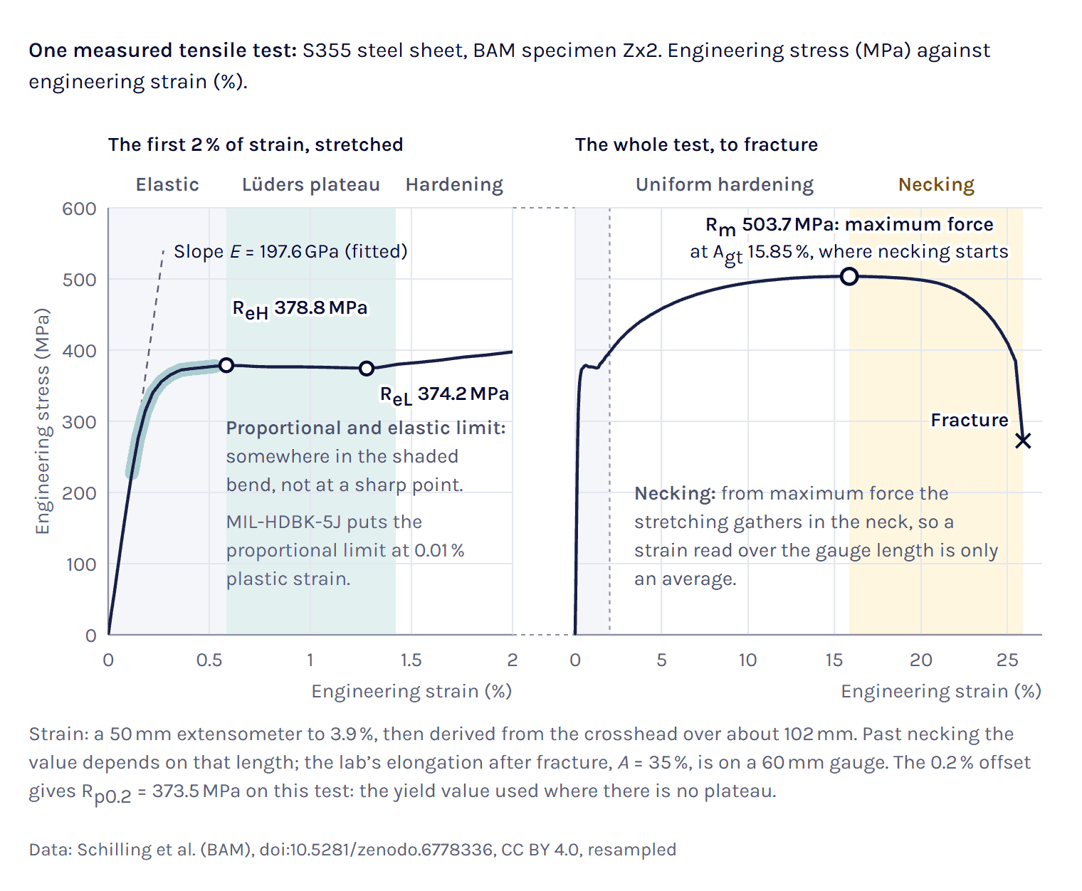
Elastic region. The straight line from the origin, where stress is proportional to strain and the specimen springs back when unloaded [3].
Yield. This steel has a sharp yield point: the stress peaks at the upper yield strength ReH, drops to the lower yield strength ReL and runs almost flat to the Lüders plateau end at about 1.4 % strain while yielding spreads along the gauge length in Lüders bands [4, 5]. Most aluminium alloys, stainless steels and high-strength steels yield gradually instead [6, 7].
Strain hardening. The metal gets stronger as it deforms, but the slope keeps falling [8] until the force reaches its maximum. That maximum over A0 is the tensile strength Rm [7], 503.7 MPa here at 15.85 % strain.
Necking and fracture. From the maximum force on, the stretching concentrates in a short neck, the force falls and the specimen breaks [3, 9]. On the broken pieces you measure the elongation after fracture A, 35 % here on a 60 mm gauge length, and the reduction of area Z, 58.8 % [7, 10].
Young’s modulus (modulus of elasticity)
Young’s modulus E, also called the modulus of elasticity, is the slope of the straight part, E = σ/ε [3]. It decides how much a part deflects under load, while the yield strength decides when it yields. Design codes give structural steel 210 GPa (210 000 N/mm²) [11], and aluminium alloys sit at about 70 GPa, a third of that [4].
A measured modulus need not match the handbook value. A straight-line fit between 10 and 50 % of the yield strength, the range TENSTAND recommends [4], gives about 198 GPa from the BAM record, where BAM itself reports 199 GPa [10]. A slope far below that usually means crosshead strain, which includes the stretch of the machine [12].
Elastic limit and proportional limit
The proportional limit is the highest stress at which the curve is still straight, and the elastic limit the highest stress that leaves no permanent strain after unloading, often equal or close on metals [3]. Since neither can be pinpointed on a real test, yield is usually reported as an offset value [3], and MIL-HDBK-5J puts the proportional limit at a plastic strain of 0.0001 [7].
Engineering stress vs true stress
Engineering stress divides the force by the original area A0 for the whole test, although the specimen gets thinner as it stretches. True stress divides by the area A at that moment, σt = F/A [13]. In the plastic range metals deform at practically constant volume, AL = A0L0 [3, 13], so while the gauge length stretches evenly A = A0/(1 + εe), which gives the true stress formula
σt = σe (1 + εe) (2)
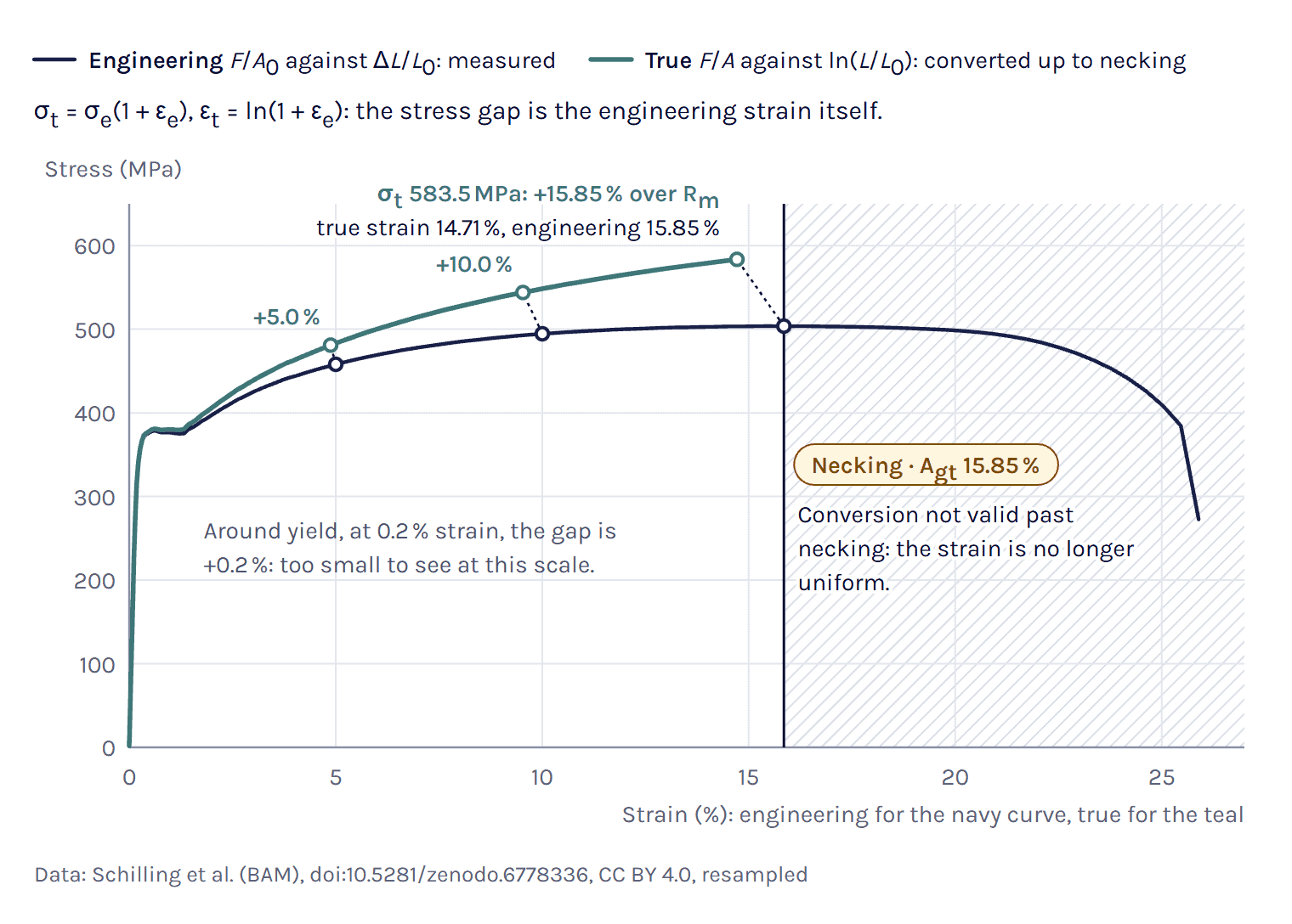
So in tension the true stress is the engineering stress times 1 + εe: 400 MPa at 20 % strain is 480 MPa true. We checked the formulas against the conversion table in the Abaqus manual, and all six of its rows come out within its rounding [14]. At the maximum force of the S355 test, 503.7 MPa at 15.85 % strain, the true stress is 503.7 × 1.1585 = 583.5 MPa, 15.85 % above Rm. At the tensile strength the true stress is always Rm(1 + Agt), so the gap equals the strain at maximum force, Agt.
The engineering and true stress–strain curves are practically equal up to the yield point: at 0.2 % strain, around the yield strain of a structural steel, they are 0.2 % apart (our arithmetic), and the difference only matters once the strain gets large [14, 15]. To plot the true stress–strain curve, convert each point of the engineering curve with (2) and (3) up to the maximum force, which is what the calculator does for a whole curve.
In compression it goes the other way: the true stress is smaller in magnitude than the engineering stress [13], so −300 MPa at −10 % becomes −270 MPa at a true strain of −0.1054.
True strain formula
Engineering strain compares every stretch with the original length L0. True strain, also called logarithmic strain, compares each small increment dL with the length L at that moment and adds them up [13]:
εt = ∫ dL/L = ln(L/L0) = ln(1 + εe) (3)
At 10 % engineering strain εt = ln 1.10 = 0.0953, and at the maximum force of the S355 test 0.1471. True strains add up where engineering strains do not: two stretches of 10 % give 2 × 0.0953 = 0.191, the same as one of 21 % (our arithmetic).
With constant volume the true strain also follows from the area, εt = ln(A0/A) [3], which still works in a measured neck: the S355 specimen’s reduction of area of 58.8 % gives about 0.89 in the fracture section, six times the 0.1471 at the start of necking.
Why the conversion stops at necking
Formulas (2) and (3) assume that the whole gauge length stretches evenly, which holds until the maximum force. After it the deformation concentrates in the neck, the stress there is no longer uniaxial, and an extensometer across the gauge length averages the neck with parts that have almost stopped stretching [3, 14]. Points converted past the maximum therefore give neither the stress in the neck nor that in the rest of the specimen.
Where necking starts follows from Considère’s construction. The force F = σtA peaks when hardening no longer makes up for the shrinking area, and dF = 0 gives [9]
dσt / dεt = σt (4)
Necking starts where the slope of the true curve has fallen to the true stress itself. The hardening rate of metals falls with strain [8], so work hardening only delays necking, and the same point is the maximum of the engineering curve [9]. The Why does necking start here? button in the calculator draws the construction on your curve.
For a power law, σt = Kεtn (the Hollomon form), necking starts at a true strain equal to the strain-hardening exponent n [3]. With n = 0.2 Roylance’s example necks at 22.1 % engineering strain, its true stress 22.1 % above the tensile strength [3].
The calculator shows the range past necking as a band, switched off by default. Its lower edge continues the Voce curve, which levels off, its upper edge is a Swift law matched to it in value, slope and curvature at necking, which keeps rising, and its middle is the mean of the two (our derivation). Any of the three can be written into the table as rows marked extrapolated, and a real material can still fall outside the band.
Yield strength and the 0.2 % offset
The yield strength is the stress at which permanent deformation starts. Steels with a sharp yield point, like the S355 above, are reported with ReH and ReL [4], here 378.8 MPa and 374.2 MPa read from the record (the lab reports ReH = 379 MPa) [10]. Altair’s help calls ReL the conservative value [5], and the calculator starts the hardening table there, since a hardening table may not drop from ReH to ReL.
For metals without a yield point the yield strength is the 0.2 % proof strength Rp0.2, often called the 0.2 % proof stress [4, 6]: draw a line parallel to the elastic part from 0.2 % strain on the strain axis, and read the stress where it crosses the curve [3]. The 0.2 % is a convention: MIL-HDBK-5J calls it an arbitrary limit that regulatory agencies accept [3, 7].
In a real part several stresses act at once, and the von Mises stress combines them into one value to compare with Rp0.2 or ReL. That check and the safety factor against yield are on our von Mises stress calculator.
Ultimate tensile strength and necking
The ultimate tensile strength (UTS), written Rm in ISO and EN test reports, is the maximum force over the original area A0 [4, 7], so it is not the highest stress the material carries: the true stress keeps rising after the maximum, and the force falls only because the neck’s area shrinks faster than the material hardens [9].
ISO 6892-1 reports give the strain at maximum force two ways: Ag, its plastic part [4], and Agt, the total, which is Ag + Rm/E (our arithmetic). For the S355 specimen they are 15.6 % and 15.85 %. The elongation after fracture A cannot stand in for them, because it includes the local stretch of the neck and depends on the gauge length [7].
Note that the calculator needs Agt to build a curve from material values. For S355 from 3 to 16 mm thick, EN 10025-2 asks for ReH of at least 355 MPa, Rm from 470 to 630 MPa and A of at least 22 %, as SCI and the steelmakers list it [11, 19, 20], with no strain at maximum force. These are specification minima, and the S355 minimum preset leaves Agt empty for you to fill in from a tensile test.
Plastic strain for FEA material input
An FE code with metal plasticity does not take the test curve as it is. Most codes want true stress against true plastic strain, the part of the strain that stays when the load is removed [14, 21], and the elastic part comes from E on the elastic material entry, so subtract it point by point:
εp = εt − σt / E (5)
The elastic part, 0.3 % strain at the maximum force of the S355 test, is not a constant, so converting each row is not the same as shifting the whole table, as the OptiStruct documentation also points out [15].
In the plastic form the first row holds the initial yield stress at zero plastic strain [14]. The plastic strain must increase from row to row [15], Radioss does not accept a falling stress [22], and the calculator keeps every table non-falling (our choice). The solver interpolates linearly between rows [14], so the calculator puts them closest together just after yield, where the curve bends most.
On a curve without a plateau the first row is the proportional limit, the stress at a plastic strain of 0.0001, as SCI recommends for stainless steel [6], listed at zero plastic strain (our choice), and Rp0.2 is a row of its own. On a steel with a Lüders plateau it is ReL as a true stress. The S355 minimum preset is the exception: it yields sharply at the specified ReH = 355 MPa, so its first row is that value, 355.6 MPa as a true stress in the plastic form and 355.0 MPa, which is also LIMIT1, in the SOL 106 engineering form (our choice).
Simcenter 3D and Simcenter Nastran
In Simcenter Nastran the elastic properties sit on MAT1 and the hardening curve on a MATS1 entry that points to a TABLES1 table [23]. TYPE=PLASTIC takes stress against total strain from (0, 0), with the second point at yield on the slope E, in SOL 106, 129, 401 and 402. TYPE=PLSTRN takes stress against plastic strain from the yield stress, in SOL 401 and 402 only [23]. The calculator’s plastic table is a PLSTRN table, and a SOL 106 deck needs the total-strain form. Note that SOL 401 and 402 leave plasticity off by default: without PARAM,MATNL,1 the MATS1 curve is ignored and the material stays linear [23], and Simcenter 3D writes that parameter from its Material Nonlinearity (MATNL) check box [26].
The STRMEAS field on MATS1 says whether the values are engineering or true, and defaults to engineering. It only matters in SOL 401 and 402 with large strain on (PARAM,LGSTRN,1), where, in solid elements, the solver converts engineering values itself and leaves values marked TRUE alone [23]. In SOL 106 a LIMIT1 that differs from the table’s yield point decides the yield strain [23], so keep the two equal. Older Simcenter 3D releases left LIMIT1 blank, which stopped SOL 106 with a fatal error [27].
In the Simcenter 3D material dialog (Manage Materials), the Mechanical page has a Stress-Strain Related Properties group, where Stress-Strain Input Data Type says what the table holds and Type of Nonlinearity chooses PLASTIC or PLSTRN [26]. The default input type is Engineering Stress-Strain, which Simcenter 3D writes for SOL 401 and 402 as STRMEAS=ENG [26]. If you paste the calculator’s true values with that default, a SOL 401 or 402 run with large strain converts them a second time. Choose True Stress-Plastic Strain for the plastic table and True Stress-Log Strain for the true total-strain form. For SOL 106, Simcenter 3D converts the table to engineering stress against total strain when it writes the deck [26]. It also writes the origin and the yield point itself from Yield Strength and Young’s Modulus and keeps only the rows past that yield strain, so set those two fields to the table’s values [26]. Its help does not say whether that rule also trims a plastic-strain table, so look once at the TABLES1 it writes.
In Simcenter Femap the curve is a function of type 13..Stress vs. Strain or 14..Stress vs. Plastic Strain, and for SOL 401 type 13 is written as MATS1 TYPE=PLASTIC and type 14 as TYPE=PLSTRN [24]. The calculator writes a type 14 function, and since the guide does not say what the true-stress types 46 and 47 write to STRMEAS [24], check the MATS1 in the written deck. Viktor Hultgren’s posts on Simcenter 3D nonlinear restarts and buckling solutions in Simcenter 3D show where the curve matters. In the second he ran the column without material nonlinearity and notes that it would likely collapse slightly sooner with it.
Simcenter OptiStruct
Simcenter OptiStruct also reads MATS1 and TABLES1 in a nonlinear subcase. TYPSTRN=0, the default, means total strain from the origin with the second point at the initial yield on the slope E, and TYPSTRN=1 plastic strain from the initial yield [15]. The engineering and the true curve are almost the same for small deformations, and large ones need the true curve [15].
Simcenter Radioss
In Simcenter Radioss the tabulated law is /MAT/LAW36 (PLAS_TAB), each hardening curve a /FUNCT of true stress against true plastic strain that starts at zero plastic strain and may not fall [21, 22]. Altair’s characterisation example converts the test curve as on this page, drops the data after necking and extends the curve linearly to 100 % plastic strain, noting that the response after necking depends on that choice [21].
Past the last row of the table
A table that ends at necking does not stop the solver there. Simcenter Nastran’s TABLES1 continues the line through its last two points [23], OptiStruct does the same unless FLAT=1 holds the last value [15], and Radioss extrapolates too [22], while Abaqus holds the last stress [14]. So one table keeps hardening in Nastran and is perfectly plastic in Abaqus. If your run goes past necking, switch on the extrapolation, which marks the added rows, and compare the band’s lower edge, middle and upper edge to see how much the answer depends on it.
Simcenter Nastran and OptiStruct have no units [23, 28], so the table must use the unit system of E and the rest of the model, MPa with millimetres or Pa with metres, while Radioss reads the units declared in /BEGIN or in a /UNIT block [29].
Worked examples
Worked example: true stress–strain curve of S355 steel
The calculator opens on specimen Zx2 from BAM’s data set on S355J2 steel sheet, a flat bar cut along the rolling direction and tested to ISO 6892-1 [10]. The extensometer came off at 3.9 % strain, so beyond that we take the strain from the crosshead, corrected for the stretch of the machine.
The preset takes from the full record E = 197.6 GPa, ReL = 374.2 MPa with the Lüders plateau ending at 1.419 %, and Rm = 503.7 MPa at Agt = 15.85 %, where the lab reports E = 199 GPa, ReH = 379 MPa and Rm = 504 MPa [10]. The 120-point sample in the calculator gives Agt = 15.48 %, because the top of the curve is flat: the stress stays within 0.5 MPa of Rm from 14.3 to 17.1 % strain. We ran Zx3 and Zx4, the other two rolling-direction specimens tested at the same speed, through the same steps and got 16.11 % and 15.67 %, so on one sheet the strain at maximum force already scatters by about 0.4 % strain. At the maximum force formulas (2), (3) and (5) give εt = ln 1.1585 = 0.14713, σt = 503.7 × 1.1585 = 583.5 MPa and, with the preset’s E, εp = 0.14713 − 583.5/197 600 = 0.1442.
The plastic table starts with ReL as a true stress, 374.9 MPa at zero plastic strain, climbs only to 379.5 MPa by the Lüders plateau end at a plastic strain of 0.0122, and ends at 583.5 MPa and 0.1442. The rows in between are model rows, from the Swift–Voce mean fitted through the test’s ReL, Rm and Agt, which is 0.3 % RMS from the record (our comparison), and the Test record example converts the record itself. The test runs on to fracture at 272.6 MPa, 0.54 Rm (our reading of the record), but none of that is in the table, so everything past 0.1442 has to come from a model.
Load the S355 test in the calculator ↑
Stainless steel 1.4301 at nominal values
Austenitic stainless steel hardens far more. The 1.4301 preset uses the EN 1993-1-4 nominal values for cold-rolled strip, fy = 230 MPa and fu = 540 MPa, with the two-stage curve of its Annex C, n = 6 and εu = 1 − fy/fu = 0.574 [6]. That curve reaches fu at 59.49 % engineering strain, so the true stress there is 861.3 MPa, 59.49 % above fu (our calculation). The table starts at the proportional limit: row 1 is 139.9 MPa true stress (139.8 MPa engineering) at a plastic strain of 0.0001, listed at zero plastic strain, 61 % of fy and inside SCI’s 40 to 70 % [6]. Annex C also limits εu to the elongation after fracture A [6], so enter A from the certificate to apply it: with A = 45 %, for example, fu is reached at 47.09 % and the true stress there is 794.3 MPa (our calculation).
Note that the measured 0.2 % proof strength of austenitic plate up to 25 mm can be 25 to 40 % above the specified minimum [6]. SCI recommends nominal values for design by FE analysis [6], but a model that has to match a test should start from the test values.
Load the stainless steel example in the calculator ↑
True stress–strain curve of aluminium 6061-T6
MIL-HDBK-5J (2003) gives A-basis values for 6061-T6 sheet along the rolling direction, Fty = 36 ksi (248.21 MPa) and Ftu = 42 ksi (289.58 MPa), values that 99 % of the material should exceed (95 % confidence) [7]. It gives no strain at maximum force, only a minimum elongation after fracture of 8 or 10 % [7], so the example uses Agt = 8 %, a value chosen for illustration.
The true stress at necking is then only 312.7 MPa, 289.58 × 1.08, 8 % above Ftu. The knee is sharp as well: MIL-HDBK-5J’s typical Ramberg–Osgood exponent for this sheet is 50 along the rolling direction and 21 across it [7], and with n = 50 the table starts at the proportional limit, 235.2 MPa as true stress and 234.4 MPa engineering, 94 % of Fty (our calculation).
References and changelog
References
[1] ISO 6892-1:2019, Metallic materials, Tensile testing, Part 1: Method of test at room temperature, ISO catalogue page (abstract). https://www.iso.org/standard/78322.html
[2] ASTM E8/E8M-24, Standard test methods for tension testing of metallic materials, ASTM International (scope). https://www.astm.org/e0008_e0008m-24.html
[3] D. Roylance, Stress-strain curves, Department of Materials Science and Engineering, MIT, 2001 (MIT OpenCourseWare 3.11 Mechanics of Materials). https://ocw.mit.edu/courses/3-11-mechanics-of-materials-fall-1999/d4ea545640f151bb66e6d8bc0ba55ed4_MIT3_11F99_ss.pdf
[4] M. S. Loveday, T. Gray and J. Aegerter, Tensile testing of metallic materials: a review, TENSTAND work package 1 final report, NPL, 2004. https://www.npl.co.uk/getattachment/2714daae-1fb4-4519-81b5-590d3b7f92c4/Test-method-review.pdf?lang=en-US
[5] Altair Radioss 2026 help (Simcenter Radioss), Material test: explicit FEA. https://help.altair.com/hwsolvers/rad/topics/solvers/rad/material_test_explicit_fea_r.htm
[6] SCI, Design Manual for Structural Stainless Steel, 4th edition, SCI publication P413, 2017: sections 2.1–2.3 and 6.4.6, Annex C. https://www.cedinox.es/export/sites/cedinox/.galleries/publicaciones-tecnicas/Design-manual-for-structural-stainless-steel-4ed-English.pdf
[7] MIL-HDBK-5J, Metallic Materials and Elements for Aerospace Vehicle Structures, US Department of Defense, 2003 (public release, superseded by MMPDS): sections 1.3.9, 1.4.1 and 1.4.4, tables 3.2.3.0 and 3.6.2.0, figures 3.2.3.1.6(a) and 3.6.2.2.6(a). https://everyspec.com/MIL-HDBK/MIL-HDBK-0001-0099/MIL_HDBK_5J_139/
[8] DoITPoMS, University of Cambridge, Mechanical Testing of Metals: Overview of plasticity and its representation with constitutive laws. https://doitpoms.ac.uk/tlplib/mechanical_testing_metals/plasticity.php
[9] DoITPoMS, University of Cambridge, Mechanical Testing of Metals: Tensile testing, necking and failure. https://doitpoms.ac.uk/tlplib/mechanical_testing_metals/necking.php
[10] M. Schilling, S. Glaubitz, K. Matzak, B. Rehmer and B. Skrotzki (BAM), Full dataset of several mechanical tests on an S355 steel sheet as reference data for digital representations, Zenodo, 2022, CC BY 4.0: data description, test protocol, tensile test results and the raw record of specimen Zx2. https://doi.org/10.5281/zenodo.6778336
[11] SCI, steelconstruction.info, Steel material properties (BS EN 10025-2 minimum values, modulus of elasticity). https://steelconstruction.info/topics/design/steel-material-properties/
[12] DoITPoMS, University of Cambridge, Mechanical Testing of Metals: Tensile testing, practical basics. https://doitpoms.ac.uk/tlplib/mechanical_testing_metals/tensile_testing.php
[13] DoITPoMS, University of Cambridge, Mechanical Testing of Metals: True and nominal stresses and strains. https://doitpoms.ac.uk/tlplib/mechanical_testing_metals/true.php
[14] Dassault Systèmes, Getting Started with Abaqus: Interactive Edition, Abaqus 2016, section 10.2 Plasticity in ductile metals.
[15] Altair OptiStruct 2026 help (Simcenter OptiStruct), MATS1 bulk data entry. https://help.altair.com/hwsolvers/os/topics/solvers/os/mats1_bulk_r.htm
[16] G. C. Ganzenmüller, P. Jakkula and S. Hiermaier, Strain measurement by contour analysis, arXiv:2211.14030, 2022, section 2.1 (the Bridgman correction). https://arxiv.org/abs/2211.14030
[17] M. G. Oliveira, S. Thuillier and A. Andrade-Campos, Inverse identification of the hardening behavior with a fully 3D virtual fields method, Advanced Modeling and Simulation in Engineering Sciences 12, 10, 2025. https://doi.org/10.1186/s40323-025-00293-7
[18] I. Dzioba, S. Lipiec, R. Pala and P. Furmańczyk, On characteristics of ferritic steel determined during the uniaxial tensile test, Materials 14(11), 3117, 2021. https://doi.org/10.3390/ma14113117
[19] British Steel, Declaration of performance, S355J2 sections to EN 10025-2, 2026. https://www.britishsteel.co.uk/wp-content/uploads/2026/01/S355J2.pdf
[20] Stahlwerk Thüringen, Structural steels according to European standard, table 3 (EN 10025-2:2019 values), 2025. https://www.stahlwerk-thueringen.de/wp-content/uploads/2025/07/Structural-steel-grades.pdf
[21] Altair Radioss 2026 help (Simcenter Radioss), RD-E 1101 Elasto-plastic material law characterization. https://help.altair.com/hwsolvers/rad/topics/solvers/rad/tensile_test_example_law_characterization_r.htm
[22] Altair Radioss 2026 help (Simcenter Radioss), /MAT/LAW36 (PLAS_TAB). https://help.altair.com/hwsolvers/rad/topics/solvers/rad/mat_law36_plas_tab_starter_r.htm
[23] Simcenter Nastran documentation, version 2606, Siemens Digital Industries Software, 2026: Quick Reference Guide (MATS1, TABLES1), Multi-Step Nonlinear User’s Guide (SOL 401 and SOL 402), and the Simcenter Nastran User’s Guide of the Femap 2412 series.
[24] Simcenter Femap documentation, Femap 2606.0001 User Guide, Siemens Digital Industries Software.
[25] G. Dhondt, CalculiX CrunchiX User’s Manual, version 2.7, keyword *PLASTIC. https://web.mit.edu/calculix_v2.7/CalculiX/ccx_2.7/doc/ccx/node232.html
[26] Simcenter 3D documentation, version 2606, Siemens Digital Industries Software, 2026: Specifying stress-strain data for nonlinear materials, MATS1 bulk entry export, Export of Nastran parameters, and Stress-strain measures and material nonlinearity (SOL 402).
[27] Siemens Support Center, KB000153430, USER FATAL MESSAGE 316 (IFPDRV) when using MATS1/PLASTIC in SOL106. https://support.sw.siemens.com/en-US/okba/KB000153430_EN_US/USER-FATAL-MESSAGE-316-IFPDRV-when-using-MATS1/PLASTIC-in-SOL106/index.html
[28] Altair OptiStruct 2026 help (Simcenter OptiStruct), Unit systems. https://help.altair.com/hwsolvers/os/topics/solvers/os/unit_systems_run_optistruct_r.htm
[29] Altair Radioss 2026 help (Simcenter Radioss), /UNIT. https://help.altair.com/hwsolvers/rad/topics/solvers/rad/unit_starter_r.htm
[30] H. N. Hill, Determination of stress-strain relations from offset yield strength values, NACA Technical Note 927, 1944. https://ntrs.nasa.gov/citations/19930081673
Changelog
October 2026: first published, with the calculator and this guide. The conversion, the curve model and the rules for FE tables were checked against the sources listed above, and the Simcenter Nastran and Simcenter 3D statements against the 2606 documentation.
Questions about stress–strain curves
Simcenter 3D
Viktor Hultgren
Application Specialist, M.Sc.
Former Altair tools
Johan Dahlberg
Application Support Specialist, Ph.D.
Choose “Technical question” in the form below and describe your case.
Ask a technical question →
How do I convert engineering stress to true stress?
Multiply the engineering stress by one plus the engineering strain: σₜ = σₑ(1 + εₑ). The true strain is εₜ = ln(1 + εₑ). For example, 400 MPa at 20 % strain gives a true stress of 480 MPa and a true strain of 0.1823. Both formulas assume constant volume and even stretching, so they hold only up to the maximum force, where necking starts. To plot the true stress–strain curve, convert each point of the engineering curve up to that maximum.
Is true stress always higher than engineering stress?
In tension, yes. The cross-section shrinks, so the same force acts on a smaller area, and the true stress is higher by the factor 1 + εₑ: by 0.2 % at 0.2 % strain and by 15 % at 15 % strain. In compression it is the other way round. The specimen gets wider, the true stress is smaller in magnitude than the engineering stress, and the true strain is larger.
What is the difference between engineering stress and true stress?
Engineering stress is the force divided by the original cross-section, F/A₀. True stress is the force divided by the cross-section at that moment, F/A. Test reports and datasheets give engineering values, such as Rp0.2 and Rm, while FE codes with plasticity at large strain want true stress against true plastic strain. Up to necking the two convert with σₜ = σₑ(1 + εₑ) and εₜ = ln(1 + εₑ).
How do you read a stress–strain curve?
Read it from the origin to fracture: the straight elastic part, whose slope is Young’s modulus E, then yield, hardening up to the tensile strength Rm, and necking until the specimen breaks. Yield comes either at a sharp yield point (ReH, then a flat plateau at ReL) or gradually, in which case the yield strength is the 0.2 % proof strength Rp0.2. The curve rises more and more slowly as the metal hardens, and after the maximum the force falls. The permanent stretch measured on the broken specimen is the elongation after fracture A.
How is a stress–strain curve measured?
In a tensile test to a standard such as ISO 6892-1 or ASTM E8/E8M. A specimen with a parallel gauge section is pulled in a testing machine, a load cell measures the force and an extensometer on the gauge length measures the extension. Strain taken from the crosshead also contains the stretch of the machine and needs a correction. The force over the original area and the extension over the original gauge length give the engineering curve.
Why can’t I convert past necking?
Because after the maximum force the specimen no longer stretches evenly. The strain concentrates in the neck, the stress there becomes multiaxial, and the extensometer averages the neck with parts that have stopped stretching. The conversion assumes even stretching, so past necking it gives neither the stress nor the strain in the neck. The curve beyond that point comes from a Bridgman correction of a measured round-bar neck, from inverse calibration with an FE model of the test, or from an extended hardening law, which is an assumption.
What plastic strain does my FEA code need?
Most codes take true stress against true plastic strain, εₚ = εₜ − σₜ/E, starting at the yield stress with zero plastic strain: Simcenter Nastran MATS1 TYPE=PLSTRN in SOL 401 and 402, OptiStruct MATS1 with TYPSTRN=1, Radioss LAW36 and Abaqus *PLASTIC. Simcenter Nastran TYPE=PLASTIC and OptiStruct TYPSTRN=0 take total strain from the origin instead. In Simcenter 3D, set Stress-Strain Input Data Type to True Stress-Plastic Strain when you paste the calculator’s plastic table (True Stress-Log Strain for its total-strain form), or a large-strain SOL 401 or 402 run converts the values a second time.
What is the 0.2 % offset method?
It defines the yield strength of a metal without a sharp yield point. Draw a line with the slope of the elastic part, starting at 0.2 % strain on the strain axis. Where it crosses the curve is the 0.2 % proof strength Rp0.2. A specimen loaded to Rp0.2 and unloaded keeps a permanent strain of 0.2 %.