Hydrostatic Pressure Considerations In Simcenter STAR-CCM+

As soon as you include gravity in Simcenter STAR-CCM+, hydrostatic pressure comes into play. Many times, you don’t need to bother – the simulation will behave as expected without further consideration. But if treated incorrectly, this part of the pressure field can be erratic, and cause unphysical results. So why is this? And when do you need to be cautious? In this blog post we will outline the details of what happens when you activate gravity in Simcenter STAR-CCM+, as well as when and why you need to take the hydrostatic pressure into consideration.

Working, piezometric and (hydro)static pressure

Let’s start by looking at how pressure is used and defined in STAR-CCM+. For numerical (and user) convenience, STAR-CCM+ uses relative pressure as both user input (e.g. boundary and initial conditions) and in the iterative solution procedure. This relative pressure is often referred to as the Working Pressure (or simply “Pressure” in the field functions) and is offset from the Absolute Pressure by the Reference Pressure (1 atm / 101325 Pa by default). The Reference Pressure is specified inside the Reference Values folder of any fluid continuum. This separation of pressures helps to avoid truncation errors in the numerical procedure, while it also (arguably) simplifies things when it comes to user input. To summarize, the relationship between the (working) pressure $P$ and absolute pressure $P_{abs}$ is

$P_{abs}=P+P_{ref}$

Furthermore, with no gravitational force present, the working pressure is equal to the static pressure, i.e.

$P=P_{static}$

However, as soon as you decide to include gravity in your simulation, the working pressure is instead referred to as the Piezometric Pressure, and the relation to the (hydro)static pressure changes to become

$P=P_{static}-\rho_{ref} \rm \bold{g} \cdot \left( \rm \bold{x}-\rm \bold{x_0}\right)$

As can be seen, the inclusion of gravity adds two important parameters: the reference density $\rho_{ref}$ and the reference altitude $\rm \bold{x_0}$ . The reference altitude is the point at which the piezometric and static pressure are considered equal.

When do you need to be cautious?

It is crucial to understand that when setting initial or boundary pressures in simulations where the gravity model is active, you are setting the piezometric pressure value. Simcenter STAR-CCM+ then calculates the corresponding (hydro)static pressure, based on the reference values you have provided. Knowing this, the first implication appears when your geometry includes pressure boundaries. For the sake of clarity, we will consider a set of examples to explain how (or if) they are affected.

Single-phase, isothermal, constant density fluid with vertical pressure boundary

Let’s consider a horizontal duct with constant density water flowing from left to right. We have an inlet boundary to the left and a pressure outlet in the far right. The pressure outlet has a specified piezometric pressure of 0 Pa. Looking at the velocity vector field we see that the flow develops symmetrically around the center axis of the duct and if we look at the (hydro)static pressure field we can conclude that it is uniformly distributed throughout the domain. In other words, the outlet hydrostatic pressure corresponds well to the internal hydrostatic pressure, already with default settings (e.g. a 0 Pa setting on the pressure boundary).

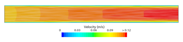
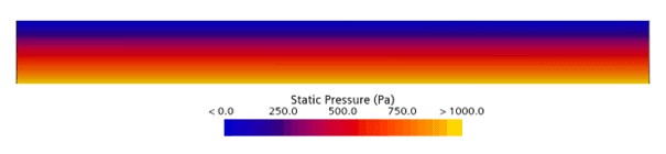
The reason for this is that for a constant density single-phase fluid, STAR-CCM+ assumes a reference density ( $\rho_{ref}$ ) identical to the material density, meaning that you do not need to specify any reference density. This way the calculated hydrostatic pressure on the boundary will always be identical to the internal hydrostatic pressure.

Single-phase, isothermal, variable density fluid with vertical pressure boundary

Let’s consider the same setup again, but this time we change from constant density water to a variable density using the IAPWS-IF97 formulation as our equation of state. Keeping all other settings as they are, we end up with the following solution:

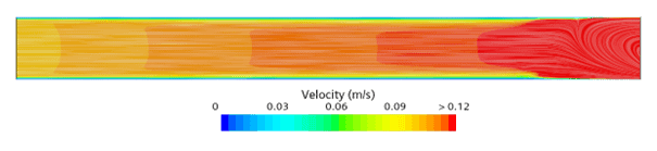
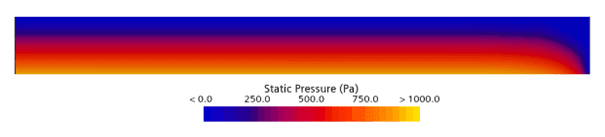
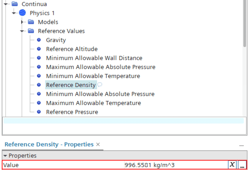
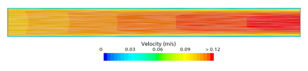
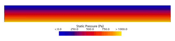
What happens here is that the calculated hydrostatic pressure on the outlet does not replicate the internal hydrostatic pressure inside the duct, causing the flow to accelerate out along the bottom end of the duct, also causing recirculation in the top. So, what went wrong here? The answer is that we did not pay attention to the reference density and altitude. The thing is, as soon as you have a variable density fluid, STAR-CCM+ assumes a reference density of 1.0 kg/m³. To make the calculated hydrostatic pressure on the outlet correlate to the internal hydrostatic pressure, the reference density must resonate with the material data. So, let’s see what happens if we update the reference density accordingly (as shown below).

Recall that the reference altitude should be the point at which the piezometric and static pressure are considered equal. The default value for the reference altitude is always [0 0 0] meters. In this case, the default reference altitude makes sense, since the domain stretches from 0 meters in the top and -0.1 meters in the bottom. This way the (hydro)static pressure will start at 0 Pa in the top (i.e. equal to the piezometric pressure at the reference altitude), and then increase with depth.

The updated result is shown in the following pictures.

We can conclude that with the correct reference values, the boundary conditions and flow behavior resonate with what we expect.

Single-phase natural convection with pressure boundaries

The differences outlined above are of utmost importance to understand when it comes to single-phase natural convection simulations with pressure boundaries. As soon as there is a connection with the ambient pressure, you need to make sure that you specify relevant reference values for density and altitude. If you do this right, the internal hydrostatic pressure will correlate to the calculated hydrostatic pressure on the pressure boundaries. This means that for a fluid with purely temperature dependent density (e.g. water, incompressible ideal gas or Boussinesq approximation), all ambient pressure boundaries should be specified with 0 Pa (i.e. zero gauge pressure) and the hydrostatic pressure will follow. Generally, these types of equation of state (i.e. purely temperature dependent densities) are sufficient for natural convection problems and are therefore the recommended practice for buoyancy driven flows.

The term “incompressible ideal gas” may be a bit confusing, but what it refers to is the assumption that for Ma ≤ 0.3 (generally the case for natural convection), the density is independent of the hydrodynamic pressure. Instead, it relies solely on the reference pressure $P_{ref}$ and the local temperature $T$ , such that

$\rho=\cfrac{P_{ref}}{RT}$

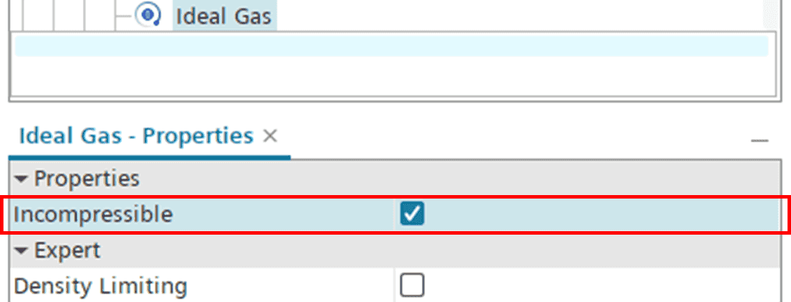
where $R$ is the specific gas constant. For the boundary condition above (i.e. $P=0$ Pa) to be valid, this option must be activated under the Ideal gas node in the continuum, see picture below.

Should you still, for some reason, choose to use a fully compressible ideal gas, the ambient pressure boundary would have to compensate for the internal hydrodynamic pressure dependence. Assuming that the ambient condition is isothermal at temperature $T_0$ , the piezometric pressure becomes

$P_{piezo}=P_{ref} \mathrm{exp} \left( - \cfrac{g}{RT_0}(z-z_0) \right) - P_{ref} - \left( -\rho_{ref}g(z-z_0) \right)$

This expression would have to be put into a user-defined field function and then used as boundary condition for all pressure boundaries. To be clear once again, this is generally not necessary and is not recommended practice, but it is included here for the sake of completeness. For full derivation of the expression, please refer to Setting the Ambient Pressure Boundary Condition in Natural Convection Cases (siemens.com).

Multiphase with phase segregation

Moving from the single-phase regime into the multiphase regime, things become a bit more complex. The added complexity arises from the fact that the multiphase regime contains more than one material density, while the pressure relation between piezometric and hydrostatic remains unchanged, i.e. dependent on a single reference density. Let’s consider again an example as the basis for our reasoning here.

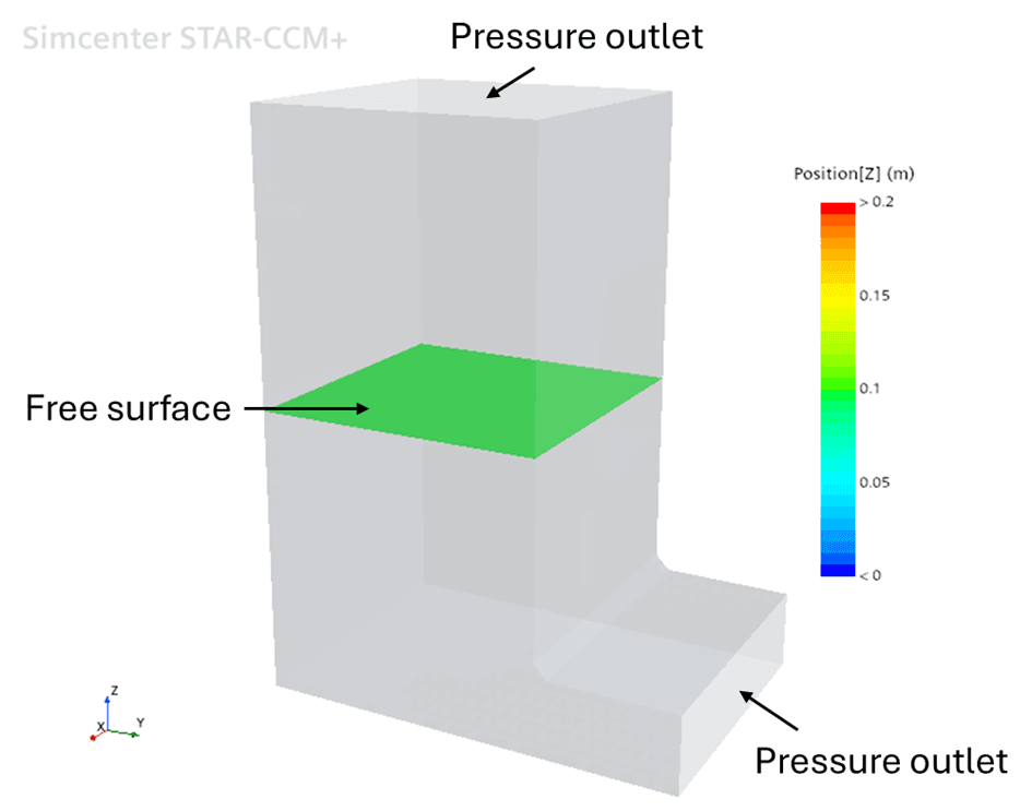
Consider a tank partly filled with water and air, respectively. The tank is 0.2 meters high, and the free surface level is set at 0.1 meters (as depicted below). The topmost boundary is open to the ambient air (and set to 0 Pa) and the rest of the tank is closed. In this example we are using the VOF model to mimic the stratified conditions.

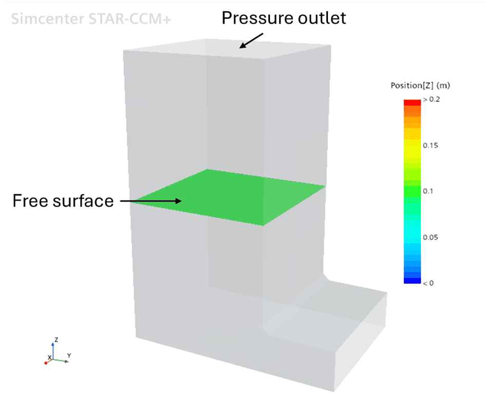
For simplicity, let’s say we have a water density $\rho_w$ of 1000 kg/m³ and an air density $\rho_a$ of 1 kg/m³. This combination together with the pressure relation basically gives us three different choices for the reference density:

$\rho_{ref}=\rho_w$
$\rho_{ref}=\rho_a$
$\rho_{ref}=0$

Let’s outline how each of the options affect the simulation.

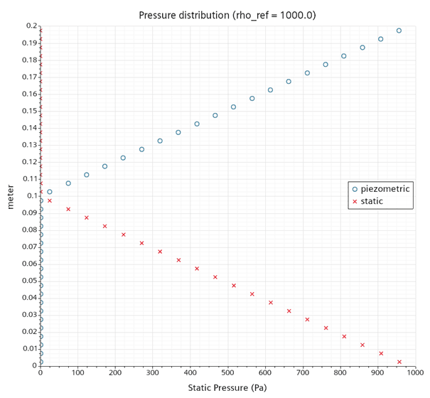
If we choose to set $\rho_{ref}=\rho_w$ , the working pressure will diminish in the water phase, but have a substantial (unphysical) gradient in the air phase. At the same time the calculated hydrostatic pressure will resonate well with the theoretical in the water phase, but differ in the air phase. The resulting pressure distribution can be seen in the plot below. Numerically, this would be an ideal situation in the water phase, but cause instabilities in the air phase.

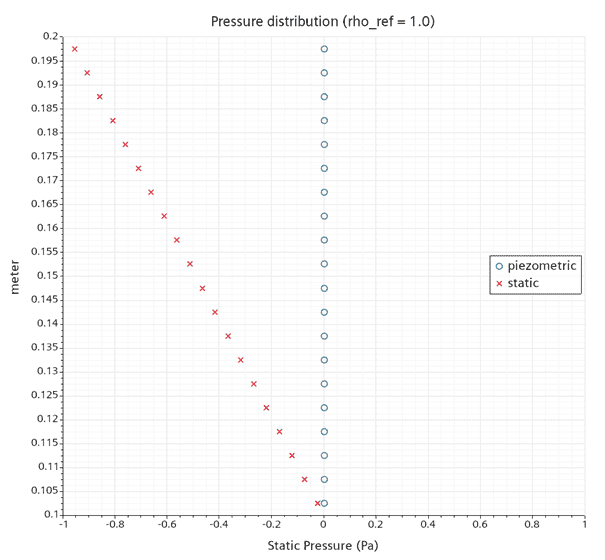
If we instead choose to set $\rho_{ref}=\rho_a$ , the working pressure will diminish in the air phase, but have a substantial gradient in the water phase. The calculated and theoretical hydrostatic pressure will be identical in the air phase, but this time have a slight discrepancy in the water phase. Below is a plot showing the pressure relation.

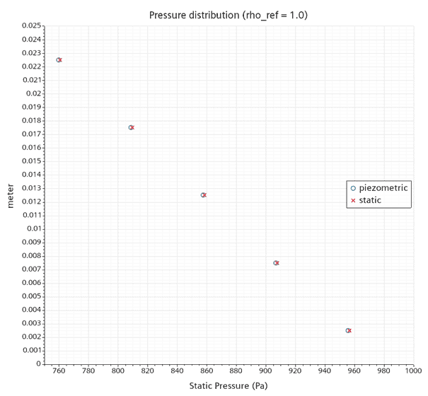
You actually need to look very closely to even see the difference between the pressures in the phases, so below you can see a couple of zoom-ins on the air pressures (top picture) and the last part of the water pressures (bottom picture). The bottom picture highlights the minor offset in pressures in the water phase. You may note that the (hydro)static pressure in the air phase has negative values. This is because the reference altitude in this case was set at 0.1 meters, i.e. the free surface level.

So, in both scenarios ( $\rho_{ref}=\rho_w$ and $\rho_{ref}=\rho_a$ ) there will be ideal numerical conditions in one-phase, and non-ideal in the other. However, with the latter option, $\rho_{ref}=\rho_a$ , the relation between the working (or piezometric) pressure and the static pressure is less problematic and will hence be the most numerically stable option of the two.

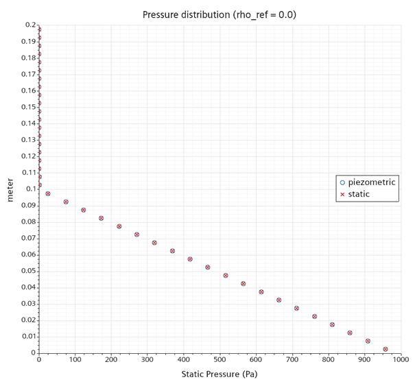
Finally, if we choose $\rho_{ref}=0$ , the working (piezometric) pressure and the (hydro)static pressure will always be identical. For the sake of completeness, you can see also this distribution in the plot below.

Based on the above, for an Eulerian multiphase simulation (e.g. VOF, EMP, MMP) where you expect phase segregation (e.g. free surface flows), the recommendation is to set the reference density to the lightest phase, or zero.

Now, to complicate things a bit more, specifying the reference density this way comes with an implication when you have pressure boundaries. Since the static and piezometric pressure on the boundaries become identical (or almost identical when $\rho_{ref}=\rho_a$ ), you can no longer rely on STAR-CCM+ to assume the correct hydrostatic pressure pillar if you set the piezometric pressure to 0 Pa (as in the single-phase regime above). This means that you need to include the hydrostatic pressure when you specify your boundary (and initial) conditions. To exemplify this implication, let’s look once again at the tank simulation – only this time we decide to include a pressure boundary at the lower side of the tank as well (as depicted below).

Let’s assume we did not know what we just learnt about the pressure relations and simply put 0 Pa on the bottom outlet. Then the hydrostatic pressure on the lower outlet boundary will also be 0 Pa (or very close to 0 Pa if $\rho_{ref}=\rho_a$ ). This type of setup would then basically imply that the lower pressure boundary is open towards the surrounding air, and the system will therefore self-drain due to the relative gauge pressure in the tank. This scenario is depicted in the animation below.

If we would rather like the free surface to be in equilibrium with a pressure boundary in the bottom, the outlet(s) must therefore include a correct representation of the hydrostatic pressure. For a horizontal pressure boundary, this pressure may well be a constant value corresponding to the actual hydrostatic pressure on that altitude. But as soon as the boundary is inclined (or vertical as in this case), it needs to include the height dependency on the hydrostatic pressure (i.e. $\rho g (z-z_0)$ ). This has to be done using a user-defined field function.

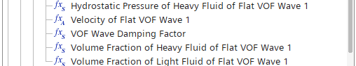
An important remark for VOF simulations, is that you can utilize the VOF Wave model to initialize your volume fraction and pressure fields. Using this model, you get a collection of pre-defined field functions ready to be used for boundary and initial conditions. This way there is no need to create your own user-defined field functions. This is actually what was used in the example above, where the pressure field was initialized with the “Hydrostatic Pressure of Heavy Fluid of Flat VOF Wave 1” field function.

You can read more about how to use this model for initialization on Siemens Support Center:

What is the best way to initialize VOF simulations?

Dispersed multiphase

The previous remarks focused on the multiphase regimes where you have distinct phase segregation, such as free surface flows. In more dilute flows, however, where you have a continuous phase and a dispersed phase (e.g. EMP, MMP, LMP, DEM) the recommendation is simply to set the reference density to the continuous phase density.

There are several articles written on this topic on Siemens Support Center, but I hope this blog post has provided a useful summary of how to treat the hydrostatic pressure and reference values for variable density and multiphase flows. If you have any questions or comments, send us an email on support@volupe.com.