Volume of Fluid (VOF) is a numerical method used in Computational Fluid Dynamics (CFD) to simulate multi-phase flows, where different fluids are present in the same computational domain. VOF is particularly useful for tracking the interface between two or more immiscible fluids. Which comes in handy for marine simulation of all kinds, but particularly when calculating the ships resistance. The VOF method is based on the idea of tracking the volume fraction of each fluid in each computational cell. Simcenter STAR-CCM+ will calculate the volume fraction of the first phase by a transport equation, representing the fraction of the cell volume occupied by the fluid. The second phase is calculated simply by subtracting the first phase fraction from 1. Please check out the blog article on Some VOF solver settings in Simcenter STAR-CCM+ to get an overview of the VOF solver settings. Here we will focus on the two finite differencing schemes and their setting for marine applications.
HRIC and MHRIC Schemes for interface reconstruction
The interface between different fluids is reconstructed based on the distribution and the movement of the interface of immiscible phases. In Simcenter STAR-CCM+ we have two sophisticated numerical approach designed to accurately capture the convective transport of immiscible fluid components with sharp interfaces, overcoming the limitations of simpler schemes, especially when dealing with varying volume fractions at the interface. The scheme incorporates blending techniques based on the normalized variable diagram to address different flow conditions.
By carefully controlling the amount of upwind and downwind differencing schemes, the HRIC scheme can produce a more accurate representation of the interface. One tuning factor is the Angle Factor (AF) controlling the blending of more or less up-wind scheme contributions into the interface capturing. The second tuning factor is the local CFL number limits to control blending of HRIC and First-Order Upwind differencing (FOU) scheme depending on the Courant number.
We have the HRIC scheme that blends with up-wind values, and we have the MHRIC scheme that blends with corrections from a quadratic up-wind interpolation (QUICK) contributions. The angle factor for this scheme is constant at 0.5. This means that for a relatively large range of angles, a significant amount of QUICK contributions are blended in.
Angle Factor
So, what is the angle factor, you may ask.
To obtain the corrected normalized face values of the volume fraction, both HRIC and MHRIC use a blending function to combine the normalized compressive face value with the corresponding correction.
![]()
This function depends on the angle between the interface and cell face normal. To know the orientation of the interface is fundamental for the application of correction. Because basic higher-order schemes, such as the central differencing scheme (CDS) or second-order upwind scheme (SOU), may fail in approximating large spatial variations of phase volume fractions. The downwind scheme is effective in sharpening the front of the interface when it is perpendicular to the flow direction. However, when the interface is parallel to the flow direction, the downwind scheme may cause wrinkling of the interface.

The angle determines practically the differencing scheme.
Example: theta=90degree to bold{F}(theta) = cos(theta)^{C_theta}=0 For which leads to a dominance of the first-order upwind scheme which avoids wrinkling of the free surface but increases the risk to be too diffusive.

The user can similarly adjust the scheme contribution using the angle factor .
Example: C_theta=0 to bold{F}(theta) =1 which leads to dominance of the downwind scheme that sharpens the free surface but increases the risk for unwanted deformation.
The MHRIC scheme uses angle correction of as well, but the angle factor has a constant value of 0.5 such that . It uses the downwind scheme much less than the HRIC due to a Downwind limit. This results in a smoother but more smeared free surface.
CFL Correction
The calculated face values are further corrected. The correction based on the local Courant number is related to the availability criterion. The availability criterion ensures that the amount of one fluid convected across a cell face during a time-step is always less than or equal to the amount available in the upstream cell.
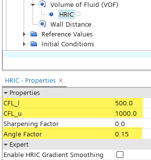
The upper and lower limit for the CFL number (CFL_u and CFL_l) are introduced to manage the blending of different numerical schemes (HRIC and FOU) depending on the Courant number in transient simulations. For CFL < CFL_l HRIC scheme is uses. For CFL > CFL_u FOU is used.
The selection of these parameters significantly impacts the stability, convergence, and accuracy of the simulation, especially in areas with high Courant numbers. In simulations where a steady-state solution is sought, such as in calm water resistance calculations, it is desirable to employ the HRIC scheme regardless of the time-step. This allows for downwind blending to enhance the sharpness of the free surface. Therefore, we set CFL_l and CFL_u to values greater than the CFL to achieve this effect.
KCS test Case
On the KCS test case we can observe the effects quite clearly. To compare the effects, we run a calm water resistance calculation with the VTT template (VTT blog). The default settings are to force the CFL correction to utilize the HRIC or MHRIC scheme with high values of CFL_l and CFL_u. We get as expected a sharp yet wrinkled interface in the figure (A) below as the result of a smaller Angle Factor (AF=0.05). In this case, the downwind scheme dominates.
In both cases where we used more upwind scheme, either through a higher AF or the MHRIC (B and C), we get a smoother but more smeared interface. It is also obvious that the deformation abates as an effect of the upwind scheme having trouble capturing large spatial variation.

In the case when we push the usage of the upwind scheme too hard, that is when we blend less with the HRIC scheme because the CFL_u limit is too small, we get a diffuser interface (see below) and even less surface elevation (D, above).

As we set sail into the world of marine free surface flow simulations, I truly hope this deep dive into the nuances of HRIC schemes sheds light on the path to enhanced accuracy and innovation. Let’s ride the waves of knowledge together and let me know your questions or comments suppor@volupe.com
The Author
Florian Vesting, PhD
Contact: support@volupe.com
+46 768 51 23 46