Simcenter Physics AI is an Altair software, now included in the Simcenter Portfolio, based on Geometric Deep Learning (GDL). This tool can predict fast solutions via machine learning, trained with simulation data. The algorithm builds models from the simulation data and does not consider the physical laws behind the results – providing a software that can be used over all simulation areas – independent of physical background. Therefore, Physics AI can be combined with all different physical simulations, as a plug-in to HyperMesh.
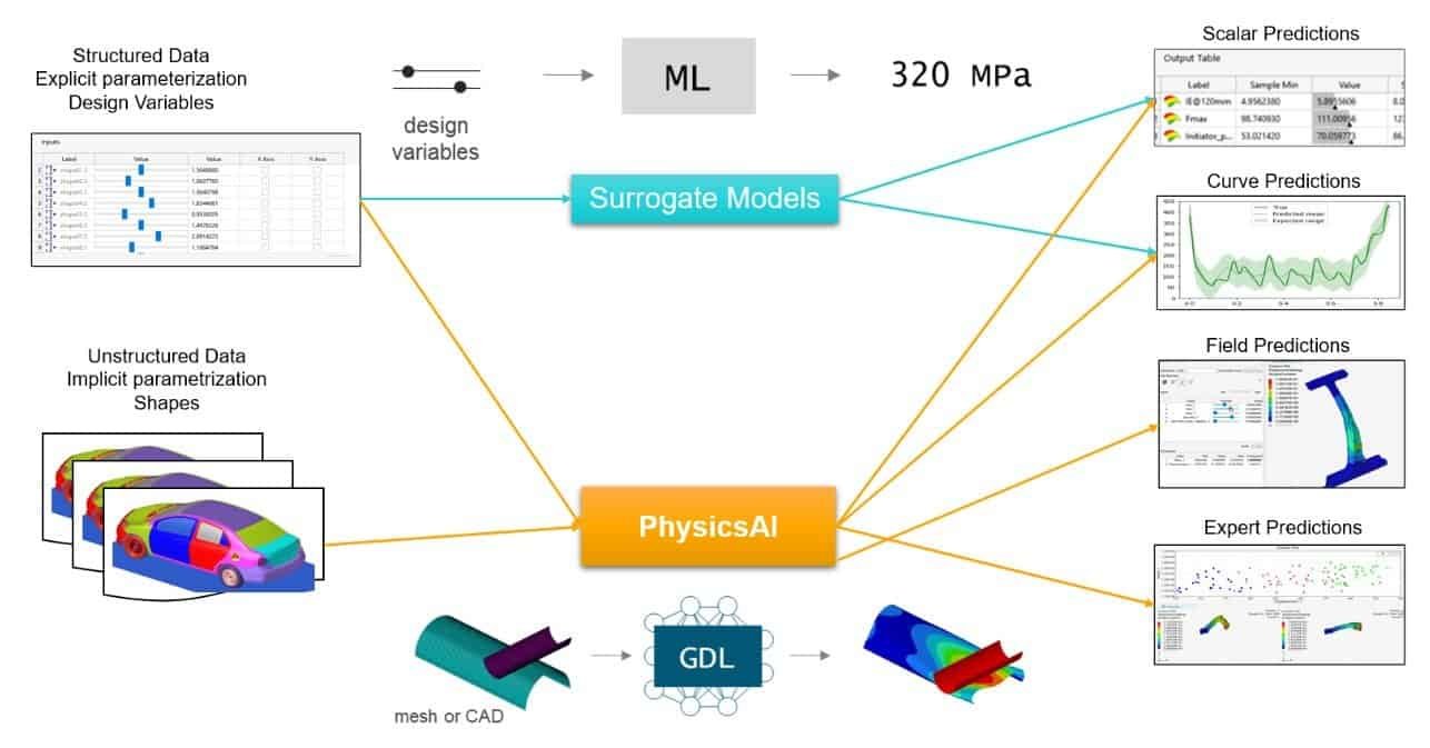
In the picture below you see another great benefit of using Physics AI compared to traditional Surrogate models and reduced order models (models you can read more about in this previous blog post: https://volupe.com/simcenter-amesim/time-dependent-neural-networks-with-simcenter-amesims-rom-builder/). Where Surrogate models are great at providing specific estimated results from structured datasets with explicit variables, Physics AI will in addition to this provide field data predictions even if the data is unstructured and no explicit design or physical properties are provided as input to the study. This gives you the possibility to predict results for new designs without the need for defining parameters, since the GDL algorithm will identify the important simulation features itself. In this way, your new shaped design will obtain predicted scalar and fields without hard-coding the parameters.
In this blog post we are describing the workflow in Physics AI, based on simulation data provided from a study in Simcenter STAR-CCM+.
Description of the Simcenter STAR-CCM+ study
The following example was created to show the workflow in Physics AI, and how to use simulation results from a Simcenter STAR-CCM+ study to train the model. The parameterization method used in the example provides the possibility to obtain results using Design of experiments instead – therefore not showing all benefits of Physics AI.
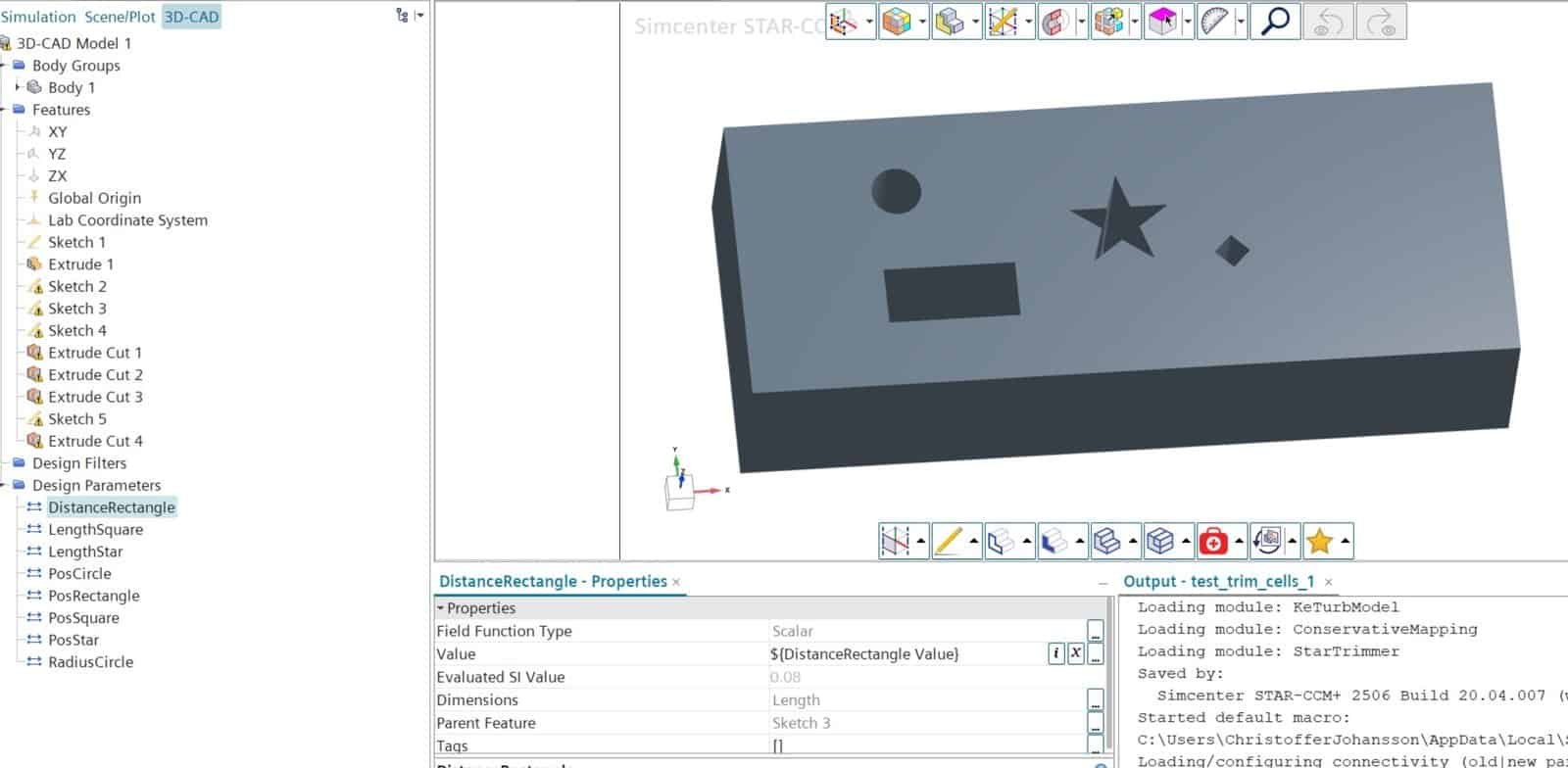
In this study, the fluid domain is represented by a block with fluid flow from left to right. Obstacles in the form of different geometrical shapes go through the fluid domain and make the cross-sections in height identical. The symmetry boundary condition on the top and bottom surface mimic an infinitely high domain. As displayed in the picture below the fluid domain is parameterized with geometrical shapes with varying locataion and size.
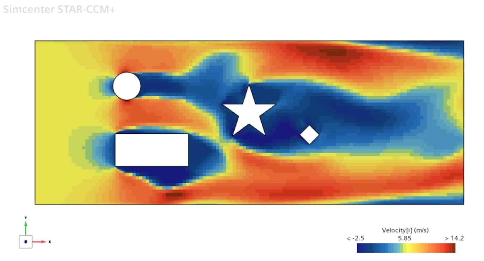
For the mesh, trimmed cells are used, since polyhedral cells are not compatible with Physics AI yet. See the picture below for a velocity result at a cross-section of the infinitely high fluid domain.
Simulation operations were used to extract results from simulations based on different combinations for the shape parameters. Using a java-macro in Simulation operations can be a good alternative to Design manager (which could have been used instead). Follow the link below for an example on how to combine Simulation operations with java scripting in Simcenter STAR-CCM+.
https://support.sw.siemens.com/en-US/product/226870983/knowledge-base/KB000045968_EN_US
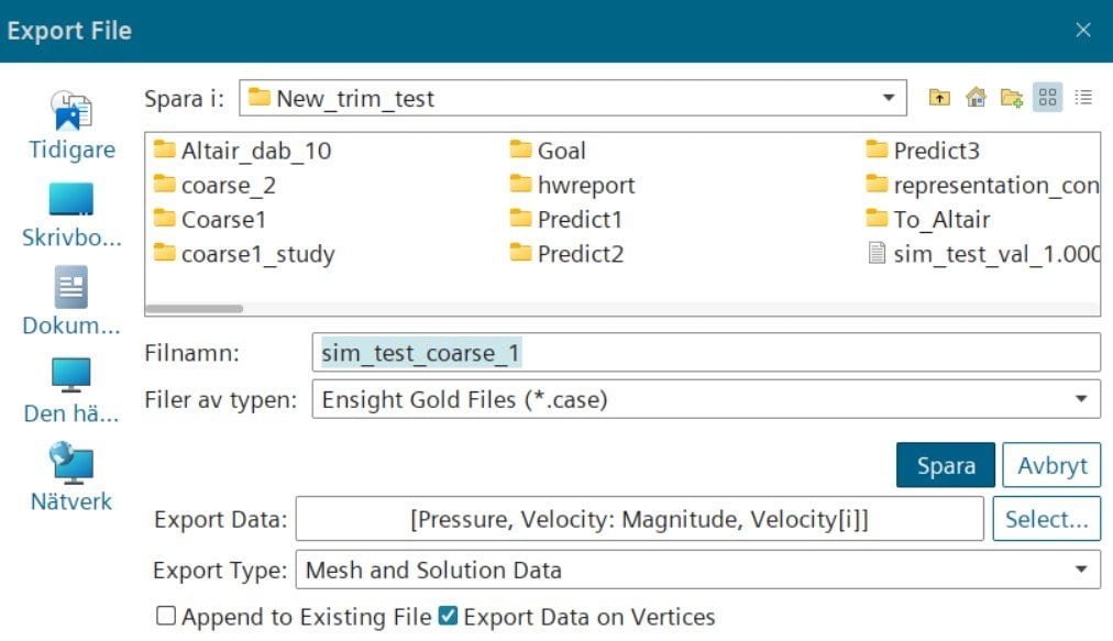
The export to .case files was handled in the java macro, where pressure and velocities were exported together with geometry and mesh. The export format .case was chosen since this format is compatible with HyperMesh, as seen below.
Physics AI workflow
In the Simcenter Altair portfolio there are many simulation software available. Physics AI is compatible with several of these software (HyperMesh, HyperStudy, HyperView etc.), and we will use HyperMesh in this study.
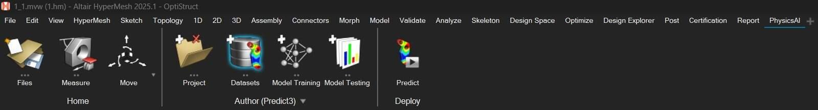
Add the tab for PhysicsAI by enabling View -> Ribbons -> PhysicsAI. Providing the toolbar menu like in the picture below. Here you can manage your project, dataset, training of your model as well as testing, and also predict results from your machine learning model.
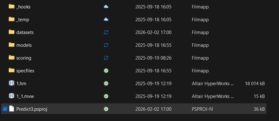
A file structure like in the picture below will be generated when creating a project. The .psproj file together with the .hm and .mvw files will be storing all project settings, and then there are specific folders for the model you develop.
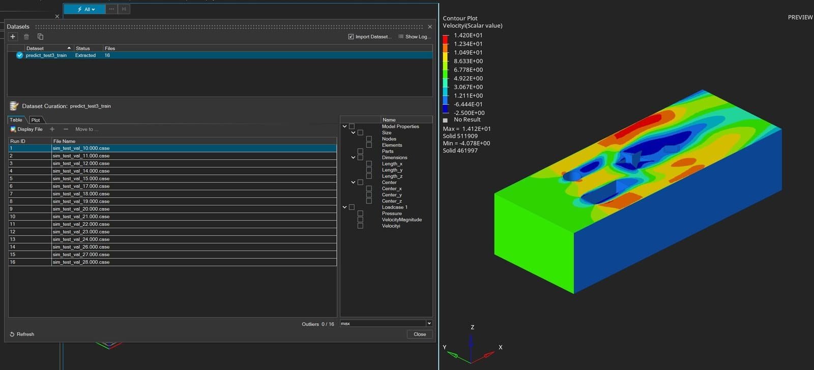
Creating a dataset is an important step in every machine learning model. This is the first step in Physics AI, and here we will refer to the data generated in Simcenter STAR-CCM+. Select the correct file format and send the desired files from left to right in the pop-up window shown below. Extracting solid faces will provide you with a model using surface data only, in this example we will tick out this box to work with volume data.
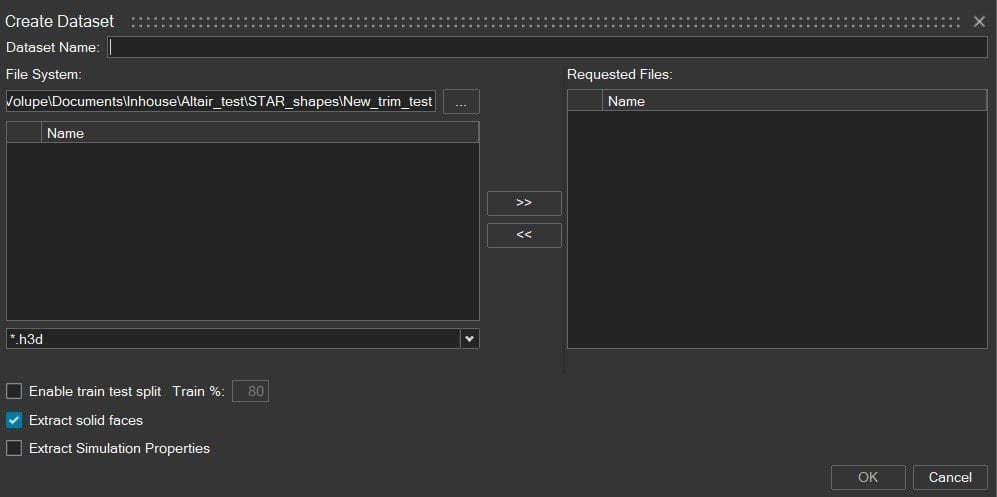
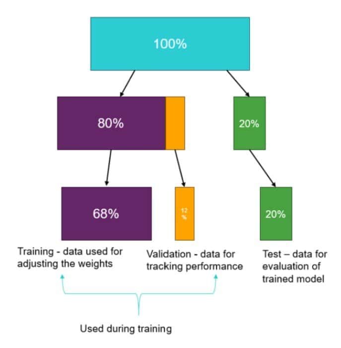
A manual training split of your dataset can be performed as well, with the “Enable train test split” option in the picture above. The default value of 80% is recommended though, and in the picture below you see how the training-validation-test data split is divided when using the 80% split.
One strength of Physics AI is that models can be generated and predict accurate results even with a small dataset. A set of 10 simulations can be enough to get an accurate model, but of course, more data to train on will provide an even more relevant/accurate model – which can be worth considering depending on which type of physics involved and the complexity of the design changes.
When the dataset is imported, you can visualize the results by Display files in Physics AI.
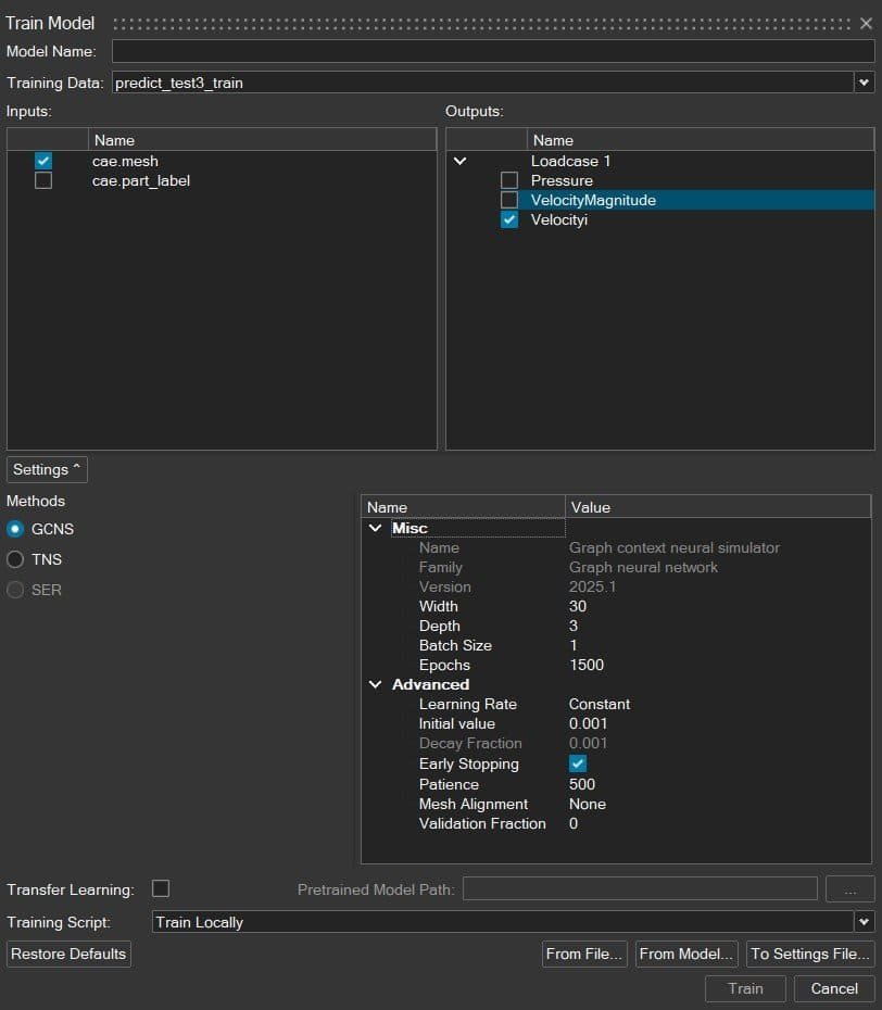
For the model training, you will set up the output and settings as shown in the picture below. The first 68% of the dataset will be used for this training.
For the output variable, it is recommended to keep the physical goal variables as few as possible. Ideally, you have one model per physical feature and make sure not to have more than three – to ensure that the model predicts as accurate results as possible for your selected variable(s). In this example, we focus on velocity in x-direction (Velocity[i]).
When it comes to model settings, we have four important values that we need to define, and this will define how thoroughly we want to create our model. The accuracy of a model always depends on how good/relevant data we have in our dataset for the specific problem we want to solve, but fine-tuning the model is done via these parameters:
- Width: Number of features of the model that are learned at once (geometrical or physical features it can keep track of).
- Depth: Number of parameters learned in a model, more parameters provide more complex models.
- Batch size: Number of training samples sent into the model at the same time.
- Epochs: The number of iterations which the model is run before it is complete (the number of times running through the dataset).
Note that increasing these parameters will make the creation of your model much slower. It will consume more RAM and take a longer time to set up the model.
When performing model training, it is a good routine to always check the corresponding Loss curve, as shown in the picture below. Where the blue line represents how much the model is changing per iteration (epoch) of fine-tuning. The star symbol indicates that a final model has been found.
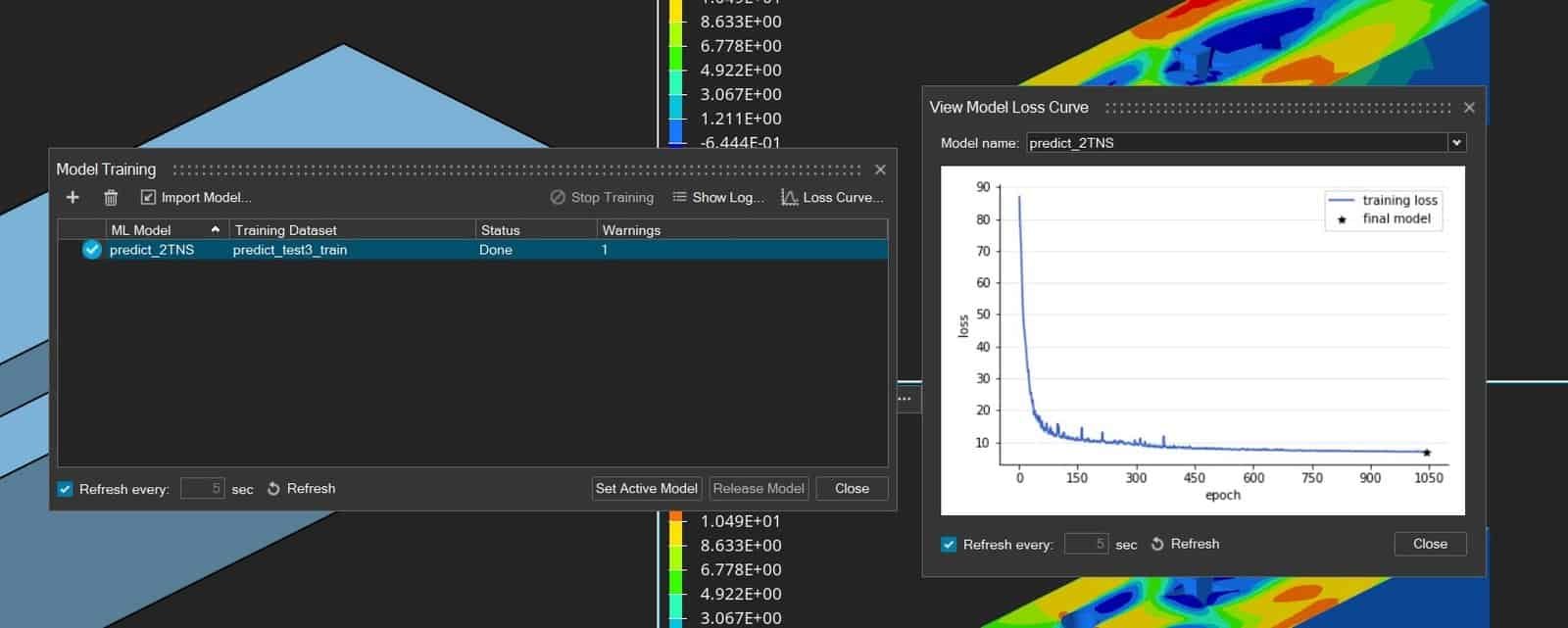
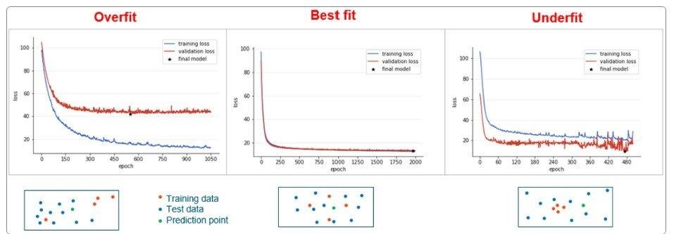
In the picture above there is no validation loss curve yet, but that would look like in the picture below. Validation loss represents how well the model performs based on the validation dataset (default 12% of the total dataset, randomly chosen). If the curves for training and validation loss decrease together and follow each other, the model will perform ideally. Overfitted and underfitted models cannot predict accurate results for all parts of the dataset. And if any of the curves don’t converge and flatten out to a lower value, your model will not be suitable to use.
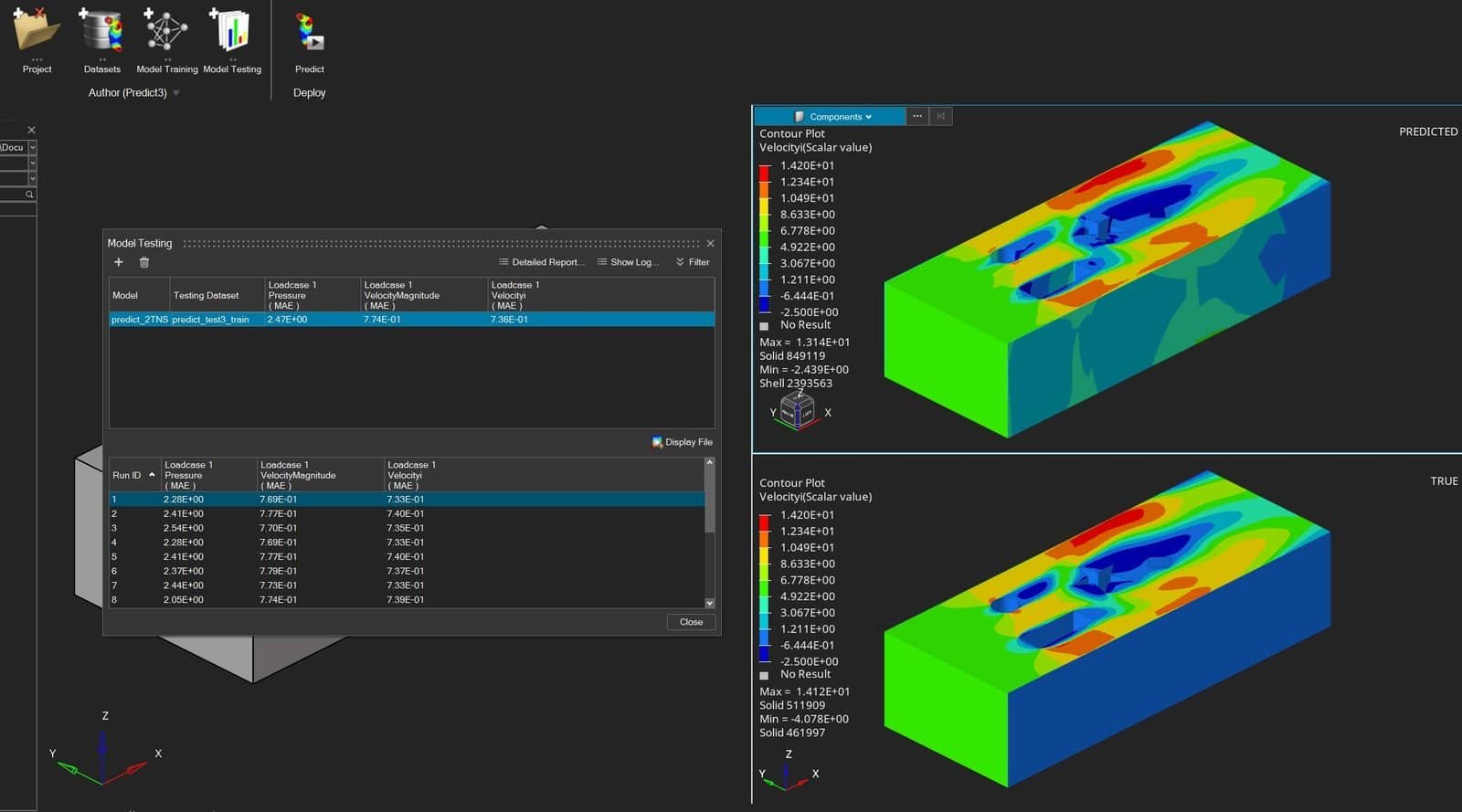
When the model is trained, you can activate the model and display predictions for the test dataset (last 20% of your dataset). In the picture below, you see a predicted result together with the true simulation results. Since physical features are not hard–coded in Physics AI, it is not surprising that the no-slip boundary condition at the wall is missed in the prediction (zero velocity at the side walls, indicated in blue color). But (most probably) this could have been predicted correctly if higher values for width, depth, batch size and epochs would have been used.
Already at the testing stage you obtain predictions, as shown above, that provide results for data not included in your dataset where the model is neither created nor validated from. To use the prediction step in Physics AI, you can obtain solutions for new geometries. In this example, we import a similar geometry with different parameter values (location and size of the obstacles). See the picture below for the predicted results which are performed in HyperMesh mode (not available in HyperView). If you have a similar tessellation/mesh resolution, you can use the similarity score as well, to get a measurement of the accuracy of the prediction. The similarity score goes from 0 to 1, where 0 indicates a prediction that is not trustworthy, and 1 would be a training datapoint (giving 100% confident result). A negative value, as in this study, is not valid. This is due to the fact that the mesh is not created to be of the same type in this example – but the eye can tell that the prediction makes sense (except for the no-slip condition at the wall as discussed previously).

This concludes the demonstration of a Physics AI workflow, and how to use results from Simcenter STAR-CCM+ as data for the GDL model. We at Volupe hope that this has been interesting and show how you as a simulations engineer can use AI in your daily work. If you have any questions regarding Physics AI, you are welcome to reach out to us at support@volupe.com. And when it comes to AI for simulations, this is just the beginning, so be prepared to see more features and possibilities based on AI included in the Siemens Simcenter portfolio in the future 😊
Author
Christoffer Johansson, M.Sc.
support@volupe.com
+46764479945