In this week’s Volupe blog post we will look at the new SIMPLEC implicit unsteady scheme and compare it to the SIMPLE scheme. The SIMPLEC scheme was introduced in version 2302 and is said to help with convergence in some cases. This is in terms of both faster and deeper convergence. We will see how the feature is presented, and we will also test this new model out in our own case. There will be a theoretical discussion about the different implicit unsteady schemes, so that we understand what is happening in the background.

We will test this out in a DNS (direct numerical simulation) case. The reason for this is to show in what capacity we can do a DNS simulation in Simcenter STAR-CCM+ and moreover how it is done.

Segregated Flow solver

Before looking at the separate schemes we require some background to how the segregate flow solver works and what role the temporal schemes play in this. The segregated flow solver solves the integral conservation equations of mass and momentum in a sequential manner. The non-linear equations are solved iteratively one after the other for the solution variable, such as the tree velocity directions and pressure. The pressure and velocity are coupled by an algorithm where the mass conservations constraint of the velocity field is fulfilled by solving a pressure-correction equation. The pressure-corrections equation is constructed from the continuity equation and the momentum equations such that the predicted velocity field is sought that fulfills the continuity equation, which is achieved by correcting the pressure. This method is generally referred to as the predictor-corrector approach. Pressure as a variable is obtained from the pressure-correction equation. Simcenter STAR-CCM+ implements either the SIMPLE, the SIMPLEC or the PISO algorithm for this. I will not include all of the equations for the segregated flow solver for brevity, but list the general steps that need to be taken to solve the discretized momentum equation (se picture below) with extra focus on the pressure gradient:

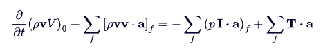
Face pressure evaluation – Pressure is part of the momentum equation in the form of a pressure gradient. To get the pressure gradient term correct, the pressure must be evaluated at each face.
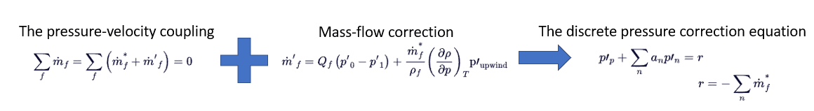
Pressure-correction equation – The pressure-velocity coupling is achieved by re-writing the continuity equation in terms of a mass flux correction.
Unsteady dissipation correction – when unsteady dissipation correction is enabled this is solved with a set of coefficients based on an acoustic CFL.
Density correction – In case of compressible flow the density needs to be corrected as well, and that is done with a density corrections term.
Discrete pressure correction equations – The discrete pressure correction equation can be obtained by combining equations from step 2 and step 4. The r here, the residual, is the net mass flow into the cell. [Residuals in Simcenter STAR-CCM+ – VOLUPE Software]

And to control the overall solution we employ the SIMPLE or SIMPLEC algorithm (or in cases with low CFL the PISO algorithm). Note that more details and equations for the segregated flow solver can be found in the documentation.

SIMPLE

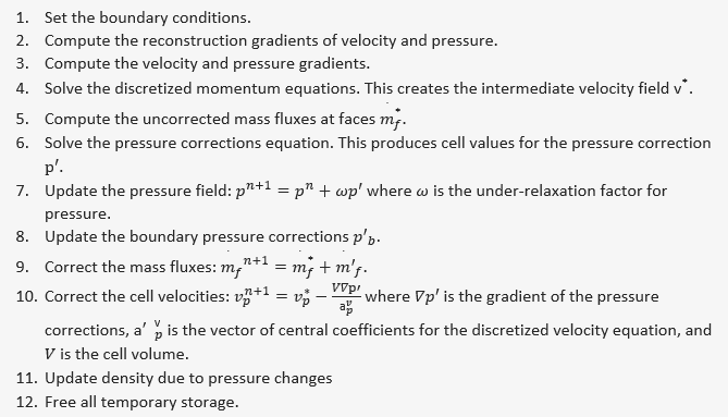
To understand the new model, we need to start by looking at the old one. It is an algorithm, and can be summarized:

SIMPLEC

SIMPLEC comes from “SIMLPE Consistent”, and it follows the same steps as summarized for the SIMPLE algorithm. The difference between the schemes is instead in the equation for the pressure correction. In SIMPLE, the velocity correction equations at a cell are first written in terms of pressure correction, neglecting velocity corrections at the neighboring cells. Taking the divergence of this equation and making use of the continuity gives the pressure correction equation.

In this velocity corrections equation, SIMPLEC assumes that the velocity corrections in the neighboring cells are equal to those at the central cells. This results in a different equation for pressure correction.

Another difference is that the pressure under-relaxation relating to the time-step size and velocity under-relaxation is implicitly built into the equation, so that there is no explicit pressure under-relaxation for the equation in point 7 under the SIMPLE section.

As a consequence of the removal of the under-relaxation factor for the pressure (effectively given the value 1), the deeper convergence is ensured within a timestep.

Siemens tested this in the DriveAer Notchback model, comparing the faster convergence to the potentially increased accuracy from the deeper convergence in each timestep.

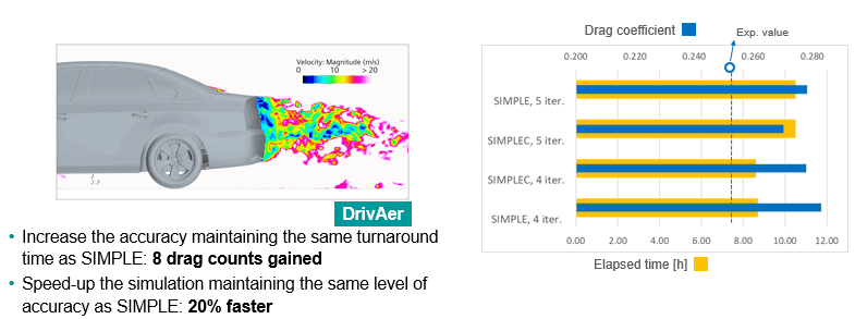
As the picture depicts, the 5 inner iterations with SIMPLE, reduced the drag count by 8 points, toward the expected value. Alternatively, the 4 inner iterations with the SIMPLEC algorithm reach the same conclusion as the 5 inner iterations with the SIMPLE algorithm. So, in conclusion, either more accurate or faster.

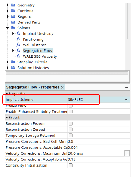
The selection for the implicit schemes is made under the solver node in the tree, under the solver for segregated flow. Note that the SIMPLEC scheme is only available for the unsteady solver.

DNS in Simcenter STAR-CCM+

Did you know that it is possible to do DNS (direct numerical simulations) in Simcenter STAR-CCM+? It is possible to perform what is referred to as quasi-DNS simulation in Simcenter STAR-CCM+. The reason it is a quasi-DNS is that a DNS simulation uses a 4^th order spatial discretization and explicit temporal integration. In Simcenter STAR-CCM+ you have access to a second order central-differencing scheme with boundedness, along with second order implicit temporal discretization. This has been shown to produce reasonable, but not fully verifiable results at the accuracy level that DNS requires.

There is no option for DNS in Simcenter STAR-CCM+ as a model selection. To run a qDNS simulation you instead need to manipulate the options for WALE subgrid scale in a LES simulation. The coefficient Cw is to be reduced to zero (1e-8). Meaning that you are adding essentially zero turbulent viscosity and solve for the laminar problem. More information on this and further recommendations can be found in this KB article on the support center [Can STAR-CCM+ do DNS? (siemens.com)].

The whole idea of this is to test the SIMPLE/SIMPLEC implicit schemes in a qDNS simulation to find out if the deeper/faster convergence can be reached according to recent claims.

The Example – flow around a cylinder

A simple example is created to do this with, the dimensions can be seen below. Due to the extremely high requirement on the spatial distribution, a quasi-2D mesh was created, a 3D mesh with only one layer of thickness. This was done using the directed mesher in Simcenter STAR-CCM+. The inlet is a velocity inlet, the outlet is a pressure outlet, and the side walls are slip walls. The prism layer consists of 20 prism layers, and the base mesh before the directed step is polygonal cells. The cell count in the case is kept at 3.7 M cells. The small cells in the refinement are about 50 microns across.

SIMPLE vs SIMPLEC results for the example

First there are some GIF-animations included of different properties related to turbulence. The pictures themselves include the entity depicted, but lets go over them anyway. Some of the different colormaps in Simcenter STAR-CCM+ have been used here. Top left picture is the velocity magnitude. The top right picture is the vorticity magnitude, in simplified terms, the rotation of the flow. The lower left picture shows the Lamb vector, the cross product of velocity and vorticity. The lower right picture shows the turbulent charge, that is the gradient of the Lamb vector.

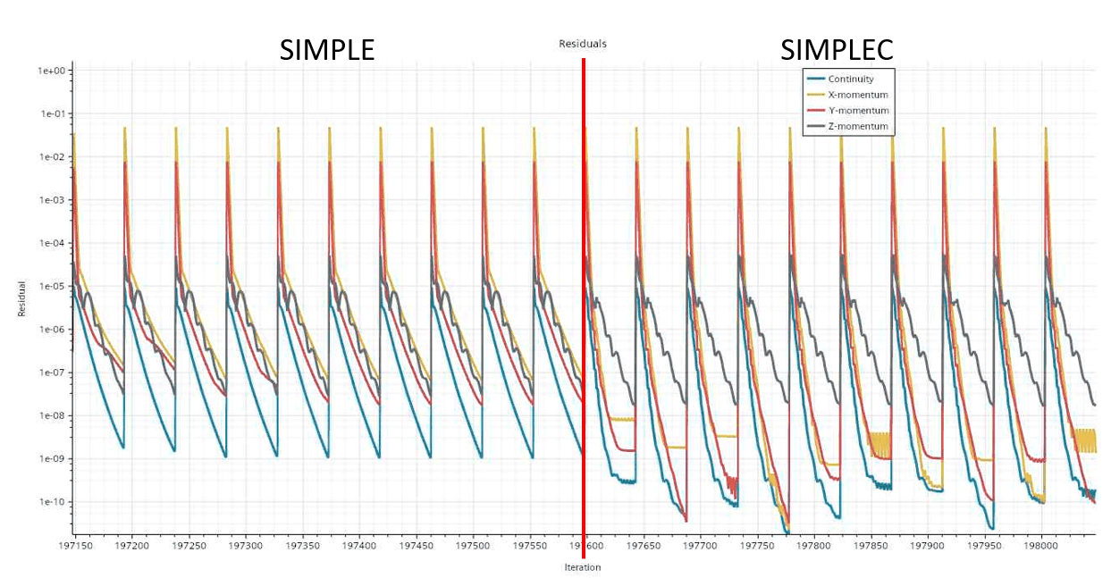
Let us take a look at what the different schemes do to the convergence in terms of the residuals, there are no experimental data or so to compare to. Since the idea of this post was to present and explain the new SIMPLEC scheme. Two comparisons were run, both at the timestep of 1e-6 s and both with a constant number of inner iterations. The picture below shows the result from when 45 inner iterations were used. It can be very clearly seen that convergence comes faster and reaches deeper in the case when SIMPLEC is used compared to SIMPLE.

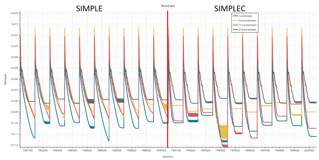
The other comparison here is with 100 inner iterations for both schemes. The total depth of the residuals for continuity is similar, but not all of the momentum residuals have completely leveled out for the SIMPLE scheme. The picture clearly shows the benefit of the SIMPLEC scheme in a case like this.

I hope that this post has been useful for you in understanding the capabilities of the new implicit scheme available for transient simulation. As usual, reach out to support@volupoe.com with any potential questions you might have.

As a bonus here is an animation of a version of the example case here. But the case in the animation is run with 1.6 M cells. It has the same number of prism layers and the same sizes, but the refinement zone for the plume is different. Let’s see if you can spot the shape of the refinement zone from the animation. We are looking at turbulent charge. The left picture is zoomed in around the cylinder and the right one shows the full domain. Note also that result shows a transition from URANS to DNS and the change of models are shown halfway in the video.

I hope that this post has been informative and helpful to you. If you have any questions, please do not hesitate to reach out to support@volupe.com.

Author

Robin Victor
+46731473121
support@volupe.com