Empirical Correlations For Convective Heat Transfer Coefficients

Empirical correlations for convective heat transfer coefficients

As a CFD engineer it is not uncommon that you encounter a problem where you need to know the convective heat transfer coefficient.
It could be a case where you need to take into account the effects of a heating/cooling flow as a boundary condition, or perhaps a case where you would like to validate (or at least make a sanity check of) your simulation results. To help you in your daily work, we decided to summarize the most commonly used empirical correlations for estimating convective heat transfer coefficients in the sections below.

The correlations are given in terms of Nusselt number, $Nu$ , which is a dimensionless property stating the relation between convective heat transfer and conductive heat transfer within a fluid. To help you even further, we have also created a Nusselt number calculator, incorporating all correlations listed on this page.

The Nusselt number definition reads

$Nu = \cfrac{hL}{k}$ (1)

where $h$ is the convective heat transfer coefficient, $L$ is a characteristic length and $k$ is the thermal conductivity of the fluid. Many generalized applications give correlations for the average Nusselt number, $\overline{Nu}$ , but some applications also allow for estimation of the local Nusselt number (i.e. based on coordinate or position on a given geometry). The average Nusselt number is defined similar to Equation 1 by simply replacing the local heat transfer coefficient, $h$ , with the average heat transfer coefficient, $\overline{h}$ .

Other dimensionless quantities needed as input to the correlations are typically the Reynolds number, $Re$ , Prandtl number, $Pr$ , Rayleigh number, $Ra$ and Grashof number, $Gr$ . You can read up on some of these quantities here: Dimensionless numbers – VOLUPE Software.

Quick access links

Click any of these links to navigate to your correlation of interest:

Natural convection

Vertical surface
Inclined surface
Horizontal surface
Horizontal cylinder

Correlations for natural convection

The following correlations have been derived for purely buoyancy driven flows (i.e. natural or free convection) and for such circumstances the Nusselt number is typically expressed as a function of Rayleigh number and Prandtl number, i.e.

$Nu = f\left(Ra, Pr\right)$ (2)

The Rayleigh number is defined as the product of the Grashof number and the Prandtl number, $Ra = Gr Pr$ . The Grashof number is a quantity describing the relation between buoyant and viscous forces acting on a fluid, defined as

$Gr_x = \cfrac{g\beta\left(T_s-T_{\infty}\right)x^3}{\nu^2}$ (3)

where $g$ is gravitational acceleration, $\beta$ is the coefficient of thermal expansion, $T_s$ is the surface temperature, $T_\infty$ is the bulk temperature, $x$ is the characteristic length and $\nu$ is the kinematic viscosity. The Prandtl number describes the relation between momentum diffusivity and thermal diffusivity and is defined as

$Pr = \cfrac{\nu}{\alpha}=\cfrac{c_p\mu}{k}$ (4)

where $\alpha = k/\left(\rho c_p\right)$ is the thermal diffusivity and $\mu$ is the dynamic viscosity. To summarize, the Rayleigh number can be thought of as an indicator of occurence of natural convection, as it relates thermal transport through diffusion to thermal transport through convection. Below a critical value of $Ra$ there is no flow and heat is transferred purely by conduction. Above this critical value natural convection is dominating the heat transfer. In most engineering problems the critical point is somewhere between 10^6 and 10^8.

Natural convection on a vertical surface

Here we consider a flat vertical hot surface (i.e.

T_s > T_\infty

) which develops a free convection boundary layer as the heated (and therefore lighter) fluid close to the wall will rise (opposite to the gravitational direction). An example of this scenario is depicted in Figure 1 below.

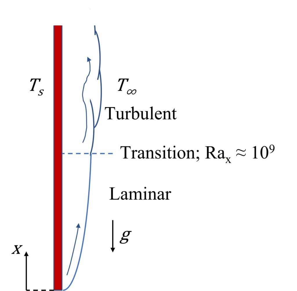
Figure 1: Natural convection boundary layer development on a vertical surface.

Churchill and Chu have proposed the following correlation for the entire range of

Ra

\overline{Nu}_L=\left[0.825+\cfrac{0.387Ra_L^{1/6}}{\left[1+(0.492/Pr)^{9/16}\right]^{8/27}}\right]^2

(5)

For purely laminar flows (typically

Ra\lesssim10^9

for vertical walls) the following relation may however give even better accuracy:

\overline{Nu}_L=0.68+\cfrac{0.67Ra_L^{1/4}}{\left[1+(0.492/Pr)^{9/16}\right]^{4/9}}

Ra_L\lesssim10^9

(6)

Please note that Equation 5 and 6 have been developed considering isothermal surfaces. Studies have however shown that these correlations can be used with good accuracy also for cases with e.g. constant heat flux (where

T_s

will vary with

x

). For such cases the

\overline{Nu}_L

and

Ra_L

should be based on the midpoint temperature on the surface, i.e.

T_s = T_s (L/2)

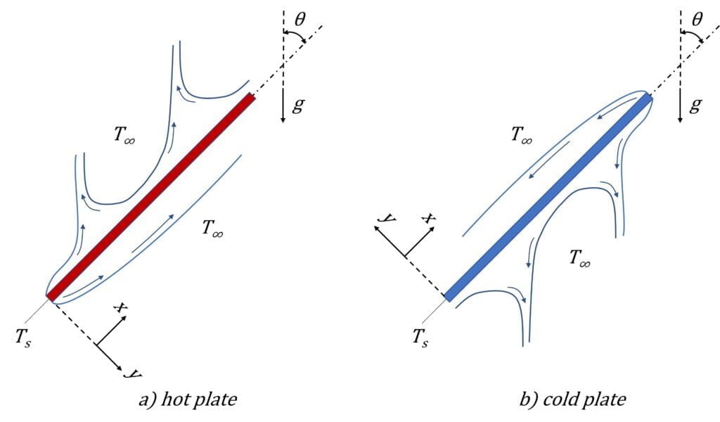
Natural convection on an inclined surface

For the case with a vertical surface the gravitational vector is parallel to surface, yielding buoyancy forces purely in the vertical direction. In the case of an inclined surface the gravitational vector becomes misaligned with the surface, yielding buoyancy forces both parallel and normal to the surface. The developed boundary layer will look different on the respective sides of the surface and also depend on whether the surface is hot or cold relative to the free stream. Figure 2 below show schematics of the boundary layer characteristics for a) a hot plate and b) a cold plate.

Natural convection boundary layer on inclined plates

Figure 2: Natural convection boundary layers on a) hot and b) cold inclined surfaces.

The characteristics of the inclined surface boundary layer obviously makes it sensitive to inclination angle, but most literature suggests that for

\theta \le 60^\circ

Equation 5 or 6 is deemed valid if replacing

g

with

g  cos  \theta

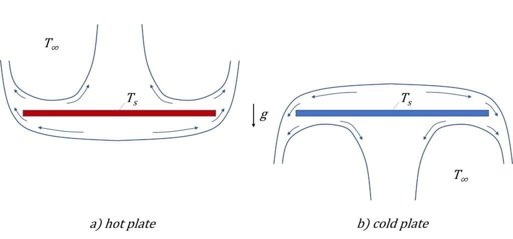
Natural convection on a horizontal surface

For horizontal surfaces the buoyancy forces instead act solely normal to the wall, but as for the inclined surface the boundary layer progression will differ for the respective sides of the surface and also depend on whether the surface is relatively hot or cold. Figure 3 shows typical boundary layers for horizontal hot plates (a) and horizontal cold plates (b), respectively.

Natural convection boundary layer development on horizontal plates.

Figure 3: Natural convection boundary layers on a) hot and b) cold horizontal surfaces.

Several suggestions on correlations exist for horizontal plates. Here we present the correlations suggested by McAdams.

Upper surface of hot plate or lower surface of cold plate:

\overline{Nu}_L=0.54 Ra_L^{1/4}

\left(10^4 \lesssim Ra_L \lesssim 10^7 \right)

(7)

\overline{Nu}_L=0.15 Ra_L^{1/3}

\left(10^7 \lesssim Ra_L \lesssim 10^{11} \right)

(8)

Lower surface of a hot plate or upper surface of a cold plate:

$\overline{Nu}_L=0.27 Ra_L^{1/4}$ $\left(10^5 \lesssim Ra_L \lesssim 10^{10} \right)$ (9)

Note that the best accuracy is achieved by redefining the characteristic length as

$L=\cfrac{A_s}{P}$ (10)

where $A_s$ is the surface area and $P$ is the surface perimeter.

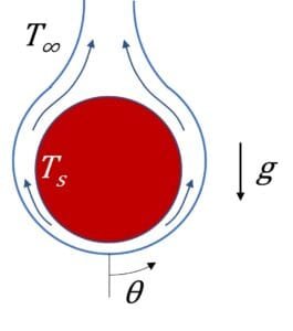
Natural convection on a (long) horizontal cylinder

The boundary layer around a heated horizontal cylinder typically forms a plume, with the boundary layer developing from

\theta = 0

at the bottom of the cylinder to

\theta = 180^{\circ}

on the top (see Figure 4 below).

Natural convection boundary layer development on a horizontal cylinder

Figure 4: Natural convection boundary layer on a long, heated, horizontal cylinder.

Extensive studies have been performed on the free convection around horizontal cylinders and as in many cases several correlations exist. One of the most widely used is suggested by Churchill and Chu and covers a wide range of Rayleigh numbers:

\overline{Nu}_D=\left[0.60+\cfrac{0.387Ra_D^{1/6}}{\left[1+(0.559/Pr)^{9/16}\right]^{8/27}}\right]^2

Ra_D \lesssim 10^{12}

(11)

Correlations for forced convection

The following correlations have been developed for cases where forced convection is the dominant factor for heat transfer and boundary layer behavior. For such circumstances the Nusselt number is typically described as a function of Reynolds number and Prandtl number, i.e.

$Nu = f\left( Re, Pr \right)$ (12)

Forced convection on a flat plate in parallel flow

Figure 5 shows a typical boundary layer formation from the leading edge of a flat horizontal plate in parallel flow.

Boundary layer development on the horizontal plate in parallel flow.

Figure 5: Forced convection boundary layer development on a heated horizontal surface.

Correlations for an isothermal plate

For an isothermal plate and a steady, incompressible, laminar flow with constant fluid properties, neglecting viscous dissipation and assuming that

dp/dx = 0

it may be shown that the local Nusselt number at a point

x \le x_c

can be expressed as

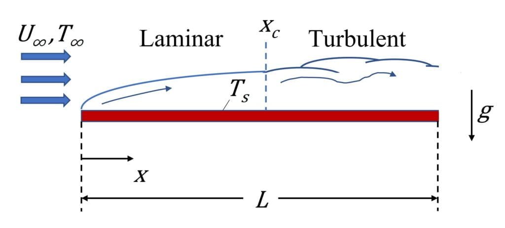
$Nu_x = 0.332Re_x^{1/2}Pr^{1/3} Pr \gtrsim 0.6$ (13)

For the same conditions, it also follows that the average Nusselt number at a point $x \le x_c$ is twice the local Nusselt number, i.e.

$\overline{Nu}_x = 2 \cdot Nu_x = 0.664Re_x^{1/2}Pr^{1/3} Pr \gtrsim 0.6$ (14)

Assuming instead that the flow has transitioned into the turbulent regime, the local Nusselt number can be expressed as

$Nu_x = 0.0296Re_x^{4/5}Pr^{1/3} 0.6 < Pr < 60$ (15)

Moreover, the average Nusselt number in the case where there are mixed (i.e. both laminar and turbulent) boundary layer conditions can be approximated by

\overline{Nu}_x=\left[0.664Re_{x,c}^{1/2}+0.037 \left( Re_x^{4/5}-Re_{x,c}^{4/5} \right) \right] Pr^{1/3}

(16)

where $Re_{x,c}$ is the critical Reynolds number where transition occurs. In a situation where $L \gg x_c$ the laminar contribution becomes negligible and Equation 16 can be simplified to

$\overline{Nu}_x = 0.037Re_x^{4/5}Pr^{1/3}$ (17)

Neglecting the laminar contribution, Equation 17 is hence also an appropriate approximation for a case where there is a turbulent boundary layer across the entire plate.

Correlations for a plate with uniform heat flux

Considering instead a situation where there is a uniform surface heat flux, the local Nusselt number for a laminar flow can be approximated by

$Nu_x = 0.453Re_x^{1/2}Pr^{1/3} Pr \gtrsim 0.6$ (18)

In the case of a turbulent flow the local Nusselt number is instead approximated by

Nu_x = 0.0308Re_x^{4/5}Pr^{1/3}          0.6 \lesssim Pr \lesssim 60

(19)

The average Nusselt number across the entire plate can be found using the following expression:

$\overline{Nu}_x = 0.68Re_x^{1/2}Pr^{1/3}$ (20)

Forced convection on a cylinder in cross flow

Another common forced convection application is the single cylinder in cross flow (see Figure 6 below).

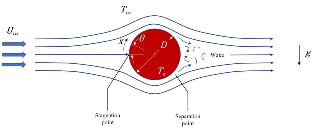
Figure 6: Streamlines and wake formation around a long cylinder in cross flow.

Churchill and Bernstein have proposed a correlation for the average Nusselt number claimed to cover a wide range of $Re_D$ and a wide range of $Pr$ . This correlation is deemed valid for $Re_D Pr > 0.2$ and reads

$\overline{Nu}_D=0.3 + \cfrac{0.62 Re_D^{1/2}Pr^{1/3}}{[1 + (0.4/Pr)^{2/3}]^{1/4}} \left[ 1 + \left( \cfrac{Re_D}{282 000} \right) ^{5/8} \right]^{4/5}$ (21)

Several other correlations exist that suggest different expressions depending on Reynolds number, aiming to account for the variation in separation point due to different flow conditions. One such widely used correlation has been suggested by Hilpert:

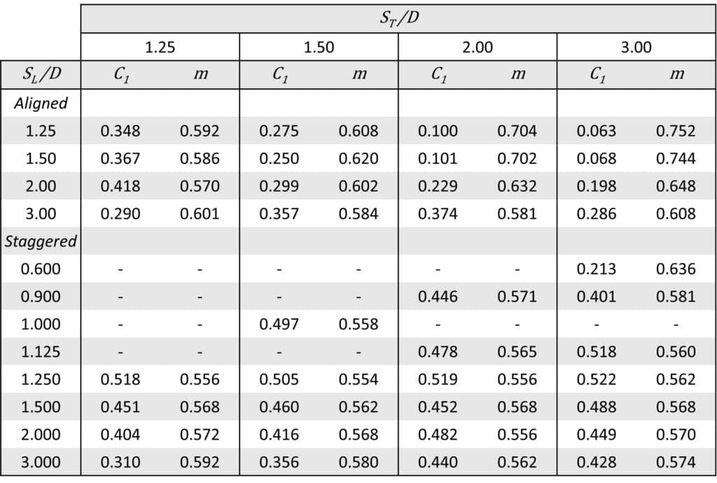
$\overline{Nu}_D = C Re_D^{m}Pr^{1/3}$ (22)

Suggested values for $C$ and $m$ are found in Table 1 below. Note that all properties used in Equation 22 should be evaluated at the so-called film temperature, i.e. $T_f=(T_s+T_\infty)/2$ .

Table 1: Constants for Equation 22.

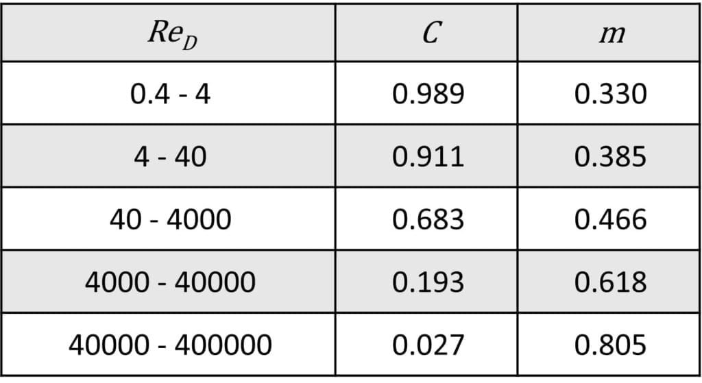
Forced convection on a bundle of tubes in cross flow

Many heat transfer applications in industry involves the flow around bundles of tubes, such as tube coolers or heat coils in boilers. The tube arrangements in such applications may vary, but typically they are either a) aligned or b) staggered. Schematic pictures of such arrangements can be seen in Figure 7.

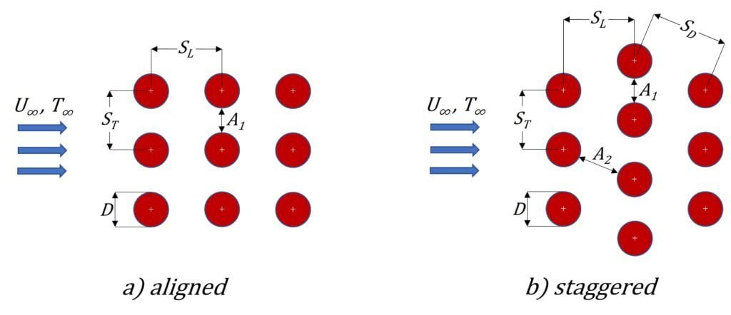
Figure 7: Cross flow on different tube bundle formations.

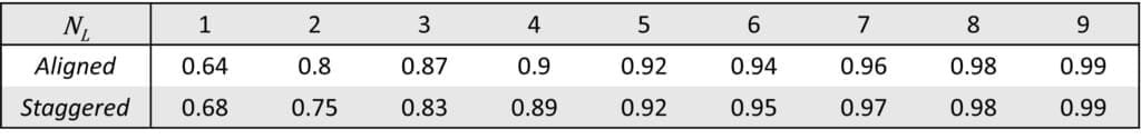
Typically, the heat transfer coefficient on the first row of tubes (normal to the flow direction) is similar to a single cylinder in cross flow. The further we move into the bundle the heat transfer coefficient tends to increase until it usually stabilizes after four or five rows of tubes. For a bundle of ten or more rows of tubes $(N_L \ge 10)$ , Grimison has proposed a correlation for airflow. To account for other types of fluids, his correlation is usually extended with a correction factor based on $Pr$ , giving the expression

$\overline{Nu}_D = 1.13 C_1 Re_{D,max}^{m}Pr^{1/3}$ (23)

which is deemed valid for the following conditions

$\begin{cases}N_L\ge10 \\ 2000<Re_{D,max}<40000 \\ Pr\ge0.7\end{cases}$

The fluid properties used in the equation above should be evaluated at the film temperature

T_f=(T_s+T_\infty)/2

. The maximum Reynolds number,

Re_{D,max}

, referred to in Equation 23 is based on the maximum fluid velocity occuring inside the tube bundle. For an aligned formation of tubes, the maximum velocity,

U_{max}

, occurs at

A_1

and assuming incompressible conditions this can be calculated by

$U_{max} = \cfrac{S_T}{S_T-D}U_\infty$ (24)

For a staggered formation,

U_{max}

will occur at either

A_1

A_2

depending on the relation between

A_1

and

A_2

. If the rows are spaced such that

2(S_D-D)<(S_T-D)

then

U_{max}

will occur at

A_2

. For such conditions

U_{max}

is given by

$U_{max} = \cfrac{S_T}{2(S_D-D)}U_\infty$ (25)

U_{max}

instead occurs at

A_1

then Equation 24 still holds. The constants

C_1

and

m

depend on the bundle formation and Table 2 below presents values for a range of different setups.

Table 2: Constants for Equation 23.

For formations with

N_L < 10

the average Nusselt number given by Equation 23 may be adjusted using a correction factor,

C_2

, such that

\overline{Nu}_D|_{(N_L<10)}=C_2\overline{Nu}_D|_{(N_L\ge10)}

or more explicitly

\overline{Nu}_D|_{(N_L<10)} = 1.13 C_1 C_2 Re_{D,max}^{m}Pr^{1/3}

(27)

Correction factors for different numbers of

N_L

are presented in Table 3 below.

Table 3: Correction factors ( $C_2$ ) for Equation 27.

For cases where the fluid temperature difference, i.e.

|T_{in}-T_{out}|

throughout the bundle is large, the Grimison correlation may not suffice. For such cases we recommend to use the correlation proposed by Zhukauskas where all properties are evaluated at the arithmetic mean of the fluid inlet and outlet temperatures. For now, the reader is referred to the literature for details on that correlation.

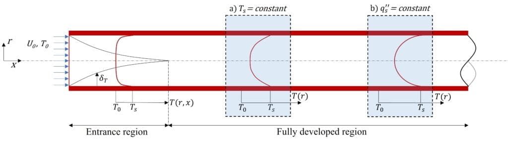
Forced convection in a circular tube

In addition to the external flow passing across cylinders or tubes (as discussed above), one may often be interested in the internal heat transfer inside the tubes. As for all convective heat transfer, the Nusselt number typically depend on the flow regime, so the following sections outline suggested definitions on the Nusselt number for laminar and turbulent flows, respectively. In addition to the flow regime, the thermal boundary layer will also depend on the wall boundary condition. Figure 8 shows a schematic overview of the thermal boundary layer development for a heated pipe, where a) refers to a case with a uniform surface temperature and b) refers to a case with a uniform surface heat flux.

Thermal boundary layer development in a heated cylinder

Figure 8: Thermal boundary layer development and temperature profiles for different wall conditions; a) uniform surface temperature and b) uniform surface heat flux.

Laminar flow

Assuming a fully developed laminar flow inside a circular tube, it may be concluded that the Nusselt number is actually constant, i.e. independent of

Re_D

Pr

or axial location. However, as mentioned above the absolute value of the Nusselt number is dependent on the wall boundary conditions. The following presents the analytical results of the local Nusselt number for cases with uniform surface temperature,

T_s

and uniform heat flux,

q^{\prime\prime}_s

, respectively.

Nu_D = 3.66          \text{if }T_s = constant

(28)

Nu_D = 4.36          \text{if }q^{\prime\prime}_s = constant

(29)

Note that for Equation 28 and 29, the thermal conductivity,

k

should be evaluated at the local mean temperature,

T_m

, defined as

T_m = \cfrac{2}{u_m r_{max}^2} \displaystyle\int_{0}^{r_{max}} uTr \, dr

(30)

where

u_m

is the mean velocity across the tube diameter and

r_{max}

is the inner tube radius. Assuming an incompressible fluid the mean velocity is given by

u_m = \cfrac{2}{r_{max}^2} \displaystyle\int_{0}^{r_{max}} u(r,x)r \, dr

(31)

For cases with a uniform surface temperature condition and a combined viscous and thermal boundary layer build-up (referred to as a combined entry length), Sieder and Tate have proposed a correlation for the average Nusselt number that reads

\overline{Nu}_D = 1.86 \left( \cfrac{Re_D Pr}{L/D} \right)^{1/3} \left( \cfrac{\mu}{\mu_s} \right)^{0.14}

(32)

which is deemed valid for

\begin{cases}T_s = constant \\ 0.48<Pr<16700 \\ 0.0044 < \left( \cfrac{\mu}{\mu_s} \right) < 9.75 \end{cases}

As stated above, this correlation is recommended for cases where the flow development in the beginning of the tube has a significant impact. This limit has been defined by Whitaker as

\left\lbrace \left[ Re_D Pr / \left( L/D \right) \right] ^{1/3} \left( \mu / \mu_s \right) ^{0.14} \right\rbrace \gtrsim 2

Below this limit, the flow can be considered fully developed and Equation 28 may be used as a good approximation for the entire tube. In the special case of a tube with an unheated starting length, i.e. where the viscous boundary layer develops before the thermal boundary layer (referred to as a thermal entry length) the average Nusselt number may instead be approximated by a correlation credited to Hausen;

\overline{Nu}_D = 3.66 + \cfrac{0.0668(D/L)Re_DPr}{1+0.04[(D/L)Re_DPr]^{2/3}}

(33)

All properties used in Equation 32 and 33 (except

\mu_s

) should be evaluated at the average mean fluid temperature,

\overline{T}_m \equiv (T_{m,in} + T_{m,out})/2

Turbulent flow

For turbulent pipe flow and assuming small to moderate temperature differences (

T_s - T_m

) the DIttus-Boelter equation is a common approximation of the Nusselt number. This correlation reads

Nu_D = 0.023 Re_D^{4/5} Pr^n

(34)

where

n=\text{0.4}

for a heated pipe (i.e.

T_s > T_m

) and

n=\text{0.3}

for a cooled pipe (i.e.

T_s < T_m

). Equation 34 has been deemed valid for the following conditions:

\begin{cases}0.7 \le Pr \le 160 \\ Re_D \gtrsim 10000 \\ L/D \gtrsim 10 \end{cases}

For cases where the temperature variation is large, Sieder and Tate have instead recommended the following equation:

Nu_D = 0.027 Re_D^{4/5} Pr^{1/3} \left( \cfrac{\mu}{\mu_s} \right)^{0.14}

(35)

with the following restrictions

\begin{cases}0.7 \le Pr \le 16700 \\ Re_D \gtrsim 10000 \\ L/D \gtrsim 10 \end{cases}

For both Equation 34 and 35, all properties (except

\mu_s

) should be evaluated at

T_m

. Moreover, both equations generally give valid approximations for both uniform surface temperature conditions and uniform surface heat flux conditions. As a final remark, additional (but arguably more complex) correlations exist, claimed to have even better accuracy (e.g. Petukhov or Gnielinski) but for now the reader is referred to literature for those equations.

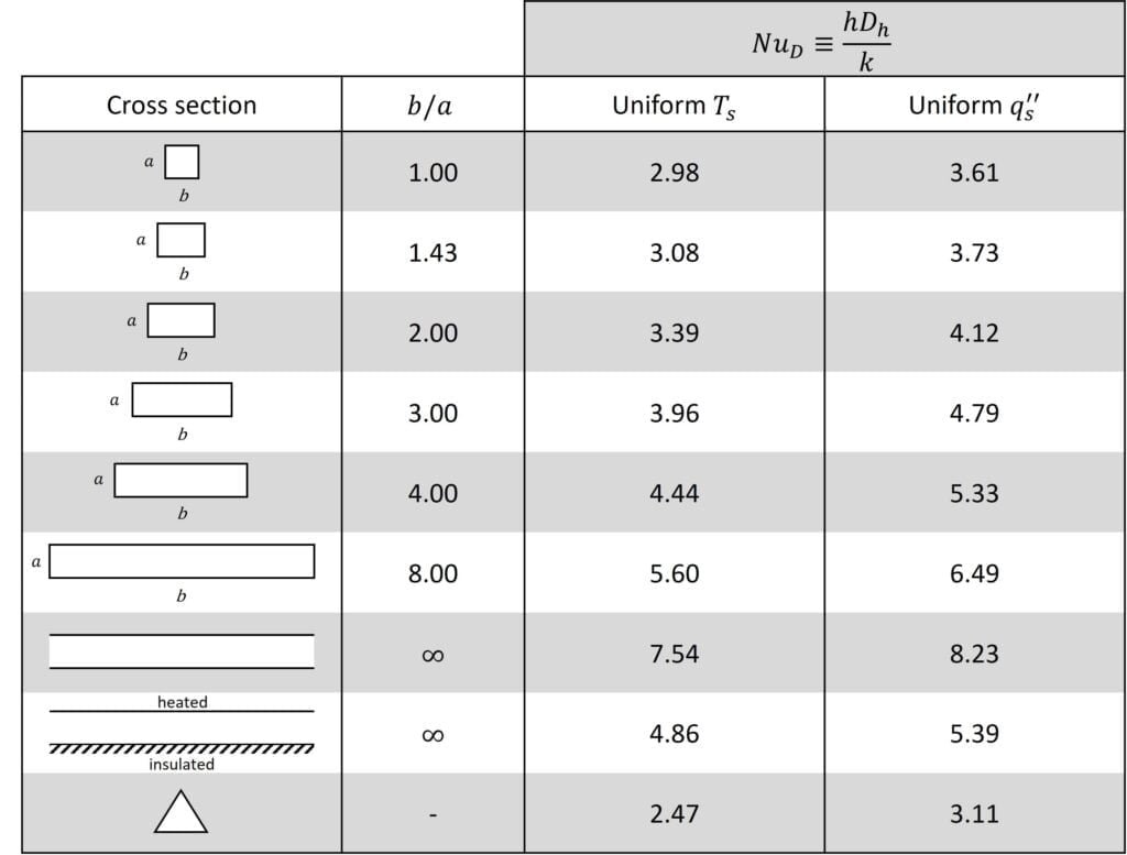
Forced convection in a non-circular duct

For turbulent flows, the correlations presented for circular tubes above may be applied also for ducts with non-circular cross sections by exchanging the tube diameter with the so-called hydraulic diameter in the calculations of the different parameters. The hydraulic diameter is defined as

D_h \equiv \cfrac{4A_c}{P}

(36)

where

A_c

is the flow cross-sectional area and

P

is the wetted perimeter. Important to note, however, is that the convection coefficients will vary along the cross-sectional perimeter and actually approach zero in the corners. Hence for non-circular ducts, Equation 34 and 35 will give approximations of the average heat transfer coefficient along the periphery.

For fully developed laminar flows, the Nusselt number can be analytically determined similar to the circular tube, but the numbers vary depending on the geometrical conditions. Table 4 below shows a collection of Nusselt numbers for a number of non-circular duct shapes, assuming fully developed laminar flow.

Table 4: Nusselt numbers for fully developed laminar flow in non-circular ducts.

Final remarks

As aforementioned, the correlations listed above are merely a selection of what can be found in the literature. For further details or alternative correlations, the reader is therefore advised to approach the available literature.

Reference list

[1] Fundamentals of Heat and Mass Transfer (5th edition), Frank P. Incropera & David P. DeWitt, 2002, USA

[2] A Heat Transfer Textbook (5th edition), John H. Lienhard IV & John H. Lienhard V, 2020, USA (A Heat Transfer Textbook, 5th edition (mit.edu))

[3] Nusselt number, Wikipedia, Accessed February 2023 (Nusselt number – Wikipedia)

Author

Johan Bernander, M.Sc.

Application Specialist

Training and mentoring for the products in the Simcenter Suit

Volupe offers training and mentoring for Simcenter products, including an introductory course for Simcenter STAR-CCM+ with basic CFD concepts. Videos on fluid dynamics and CFD are also available for users without a background in the field.