Amesim Optimization - Built-in Tools

In this Simcenter Amesim post we will have a look at the optimization features and methods available in Simcenter Amesim, and hopefully provide some insight into the field of optimization in general.

“Optimization, also known as mathematical programming, is a collection of mathematical principles and methods used for solving quantitative problems in many disciplines, including physics, biology, engineering, economics, and business.” – Britannica.com

As an engineer working with system simulation, your goal when designing a system, or component, is typically to improve on the system and enhance it as much as you can in some sense. Usually this involves comparing and cross-checking results with a large set of requirements, investigating trade-offs, and having a realistic sense of the costs involved. If the product is replacing an existing one, it needs to be at least as good as the old one, or more preferably, significantly better than the old. Other aspects involve making it ready for market in a shorter time, less expensive, easer to maintain, lower energy requirements, the list goes on. A realistic way of managing ever increasing demands and ensuring that no stone is left unturned during the development, is to leverage optimization.

Optimization in Simcenter Amesim

Setting up and defining optimization cases inside Simcenter Amesim is done through the Study Manager, figure 1. Here both independent and dependent variables are collected from the underlying Simcenter Amesim model and included under the Study Parameter Definition. Under the same folder optimization objectives, i.e. goal functions, are placed along any constraints.

Figure 1, Simcenter Amesim’s Study Manager showing a selected Optimization process

In Simcenter Amesim the following two optimization algorithms are available:

NLPQL

Genetic Algorithm

The Non-Linear Programming by Quadratic Lagrangian (NLPQL) is a gradient based algorithm for non-linear problems. The method makes use of the objective function’s gradients, or approximate gradients, to incrementally improve an objective function and is in general well suited for local searches.

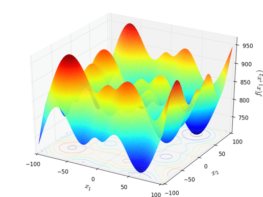
A characteristic of this gradient based approach is that it will stop once it finds a local minimum. Therefore, the final optimal solution may depend on your choice of starting point, i.e. your initial parameter values. For many optimization problems this might not be an issue since there may only be one minimum, such as for a circular paraboloid. However, if the problem is more complex in the sense that it contains multiple local optima, known as multi-modal, this algorithm may not succeed in finding the optimal solution.

As with all optimization studies, much can be gained from studying and understanding your problem before deciding on which method to use. Below in figure 2, a two-dimensional function called the Schwefel function is shown. Similar functions are used to test optimization algorithms and evaluate their behavior.

Figure 2, a two-dimensional Schwefel function containing multiple local minimums and maximums

The Genetic Algorithm inside Simcenter Amesim is what is called an evolutionary algorithm and this type of algorithm is often employed to improve the chances of finding the global optimum. The algorithm does not rely on a gradient to determine the direction of the solution. Instead it starts its wide search by randomly generating and running a set of simulation cases, much like a limited Design of Experiments (DoE) study. The result from each simulation is then evaluated, and the cases which improve the objective function the most are kept. The algorithm then continues by selecting new cases (children) from the previous cases (parents), and by choosing parameter values which are close to these parents. Each child case takes parameter values from two of the parent cases, and the optimization continues over several generations, i.e. iterations, until the maximum number of generations is reached.

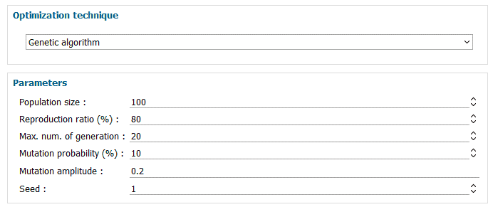
Figure 3, Default settings for the Genetic Algorithm

In figure 3 above, the settings for the Genetic Algorithm are given. Population size specifies the number of individuals/cases to run during each iteration. Reproduction ratio tells the optimizer what number of cases to be replaced with new cases in each iteration. The default value of 80 [%] means that the best 20 [%] of the cases will be kept for the next iteration. Maximum number of generations defines the total number of iterations to carry out. Mutation probability is only applied in scenarios where discrete parameters have been selected and provides the algorithm with the probability of mutating these parameters. Mutation amplitude ensures that there is room for more design exploration and limits the risk of converging on a local optimum. If values are set close to zero the solution will likely converge quicker, but with the risk of getting caught in a local optimum. Finally we have the Seed, which provides the pseudo-random number generator with a starting point. If two optimizations are run with the same Seed, and without changing any other settings, you will obtain the exact same result from both studies. If instead another Seed value is selected, then both starting point and the subsequent search will be different.

Below are some general guidelines which may help when determining algorithm settings.

The number of total simulations to run is given by the following equation.

, where N = population size, R = reproduction ratio, and G = maximum number of generations

The population size should be chosen according to the number of parameters. Experiments show that population size ≥ 4.5 x number of parameters often gives good results.

A high reproduction ratio often leads to fast convergence but is also likely to lead to a local convergence. A reproduction ratio between 50% and 85% often gives good results.

The number of generations to set depends on the number of runs you are ready to accept in term of calculation time, but it must be greater than 10 to get relevant results

Further considerations

Objective functions in Simcenter Amesim are determined by calculating the absolute value of the selected dependent variable, e.g. model output, which the optimization algorithm then seeks to minimize. This is sufficient for single objective optimization, but in situations where several objective functions are to be used, a multi-objective optimization approach is required.

When solving a multi-objective optimization problem, we are trying to find the global Pareto-optimal set. The Pareto-optimal set is the set of points where there exist no other points that are better than these points, and where any improvement made to one objective comes at the cost of the other objectives. If we plot all these points in one plot, we obtain the Pareto front/frontier, and in a scenario with two objective functions this provides the optimal trade-off curve.

At the moment no straight forward option for running Pareto optimization is in place within the Study Manager, but by combining Simcenter Amesim with Simcenter HEEDS, Simcenter’s multidisciplinary design optimization software, such an approach is possible.

An alternative to solving multi-objective problems using Pareto optimization is to define a single function from two or more objective functions and then optimize this single function. This approach is known as the weighted sum approach, and is a widely used method. The approach uses weights to specify the relative importance of each objective, and then scale the different magnitudes of all objectives using a process called normalization.

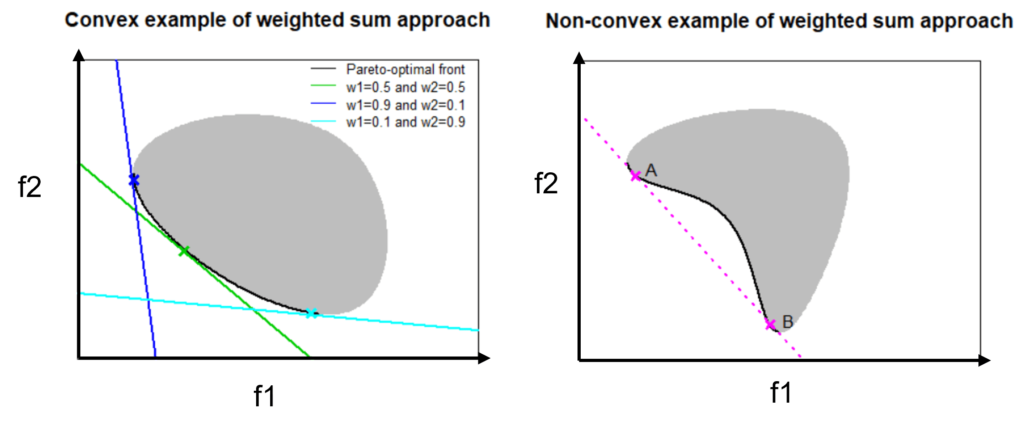
The weighted sum approach is adept at solving problems which can be classified as having a convex objective space, which is fairly common for many engineering problems. If equal weights are assigned, meaning that all objectives are deemed equally important, the weighted sum approach will find this point on the Pareto frontier. Choosing different weights will result in finding different optimal solutions on the Pareto frontier, as seen in figure 4 below.

Figure 4, left, a problem containing a convex objective space with different weights applied. The figure to the right shows a non-convex example. [1][2]

For non-convex problems as given to the right in figure 4, the weighted sum approach fails at determining optimal points between A and B. This is due to that the weights will form a line that will intersect A or B before any point in between. An optimum will still be found, however, not the best for the given weights. To find the optimal trade-offs in this situation, Pareto optimization needs to be employed.

Optimization as a subject is extensive and its applicability likewise so. In more straight forward problems, optimization can effectively be used to ascertain parameter settings of, for example, a check-valve in order to match some requirements in flow, or to match a model of a turbocharger inside Simcenter Amesim with tested results. In more advanced cases, optimization is used to determine the relationship and trade-offs between different system attributes in a complex system, containing several objective functions, numerous inputs, and more than a few constraints.

These problems can of course be approached using more heuristic methods, such as trial and error, but with the drawbacks of a less systematic workflow, no guarantees of actually finding optimality, and the great risk of leaving some very important stones left unturned.

In an upcoming blog we will go through how to connect Simcenter HEEDS with Simcenter Amesim. In the meantime, we hope you have found this article interesting. If you have any questions or comments, please feel free to reach out to us on support@volupe.com