Predicting heat transfer behavior is a fundamental aspect of thermo‑fluid system design. Whether the objective is to enhance cooling performance, evaluate thermal safety margins, or understand how temperature variations affect fluid properties, engineers require simulation tools that represent heat transfer phenomena with a high degree of accuracy.
In this article, we examine how Simcenter Flomaster supports system‑level heat transfer analysis in piping networks. We highlight how different modeling approaches and configuration options influence thermal behavior, simulation fidelity, and the quality of engineering decisions that can be drawn from the results.
Furthermore, the additional information may lead to more accurate simulation results as temperature dependent properties such as fluid viscosity are updated accordingly. In particular, Simcenter Flomaster has the ability to extensively model heat transfer within pipes, which can operate under different modes of heat transfer depending on the known thermal properties.
Modeling Pipe Heat Transfer
Simcenter Flomaster provides several methods for modeling heat transfer, allowing different levels of thermal complexity depending on system requirements. These capabilities include:
- Applying heat input or heat output to a system
- Modeling heat transfer between fluids across an interface
- Performing thermal analysis of pipe walls
- Simulating mixing between hot and cold fluid streams
- Accounting for temperature-dependent variations in fluid properties
- Modeling heat exchange between solid components and fluids
- Capturing heat transfer effects even in no-flow conditions
When a fluid flows through long pipe networks, significant heat exchange can occur between the fluid, the pipe wall, and the surrounding ambient air. This heat transfer process is typically modeled in three main stages:
- Heat Transfer from Fluid to Inner Pipe Wall
This process is calculated using a Nusselt number correlation based on the Dittus–Boelter equation given below. It should be noted that the Dittus–Boelter correlation is derived specifically for cylindrical pipes and is therefore not suitable for pipes with rectangular, hexagonal, or other non-cylindrical cross-sections.
The Dittus-Boelter Coefficients are used to calculate Nusselt number (Nu) using the Reynolds number (Re) and Prandtl number (Pr).
![]()
- Heat Transfer Through the Pipe Wall
Heat conduction between the inner and outer pipe walls is determined based on the pipe material, wall thickness, and any additional insulation layers that may be present.
- Heat Transfer from Outer Wall to Ambient
Heat loss from the external pipe surface to the environment is calculated using the surface emissivity of the pipe and the ambient temperature. Alternatively, heat transfer can be modeled as adiabatic or defined using a specified heat loss per unit length of pipe.
A selection between eight different heat transfer modeling options can be done, allowing users to select the most appropriate approach based on the available input data and the required level of modeling detail, as summarized in the table below. It is also possible to model the effects of pipes that are fully exposed to external flow, e.g. surrounding a subsea pipeline, fully buried, or partially buried/exposed.
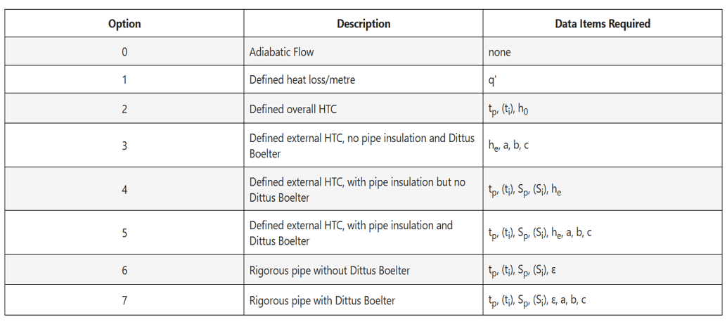
q’ is the defined heat loss per unit length, tₚ is the pipe thickness, tᵢ is the insulation thickness (if applicable), h₀ is the overall heat transfer coefficient (W/m²·K), hₑ is the external heat transfer coefficient (W/m²·K), Sₚ denotes the pipe material type, Sᵢ the insulation material type, a, b, and c are the Dittus–Boelter coefficients, and ε represents the surface emissivity.
Thermal example
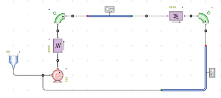
Below, a simple model of a water circuit is shown. Water is pumped from a reservoir to a heat exchanger/heater where heat is added to the system. The fluid then flows through a pipe before entering a second heat exchanger acting as a cooler where the heat is removed. In the study below the properties of the 150 [m] pipeline between the two heat exchangers are altered.
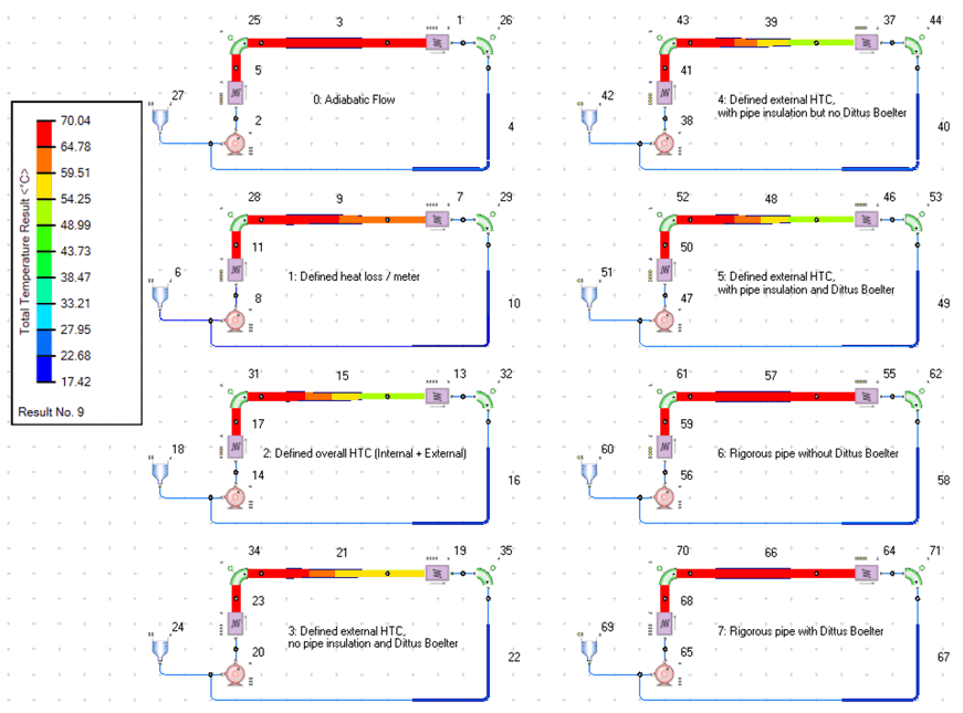
The temperature results demonstrate that the choice of model can lead to significantly different outcomes. Therefore, careful consideration is required when configuring a thermal simulation to ensure that the selected model accurately represents the physical phenomena of interest.
Another way of viewing these results is to consider temperature w.r.t. pipe length instead.
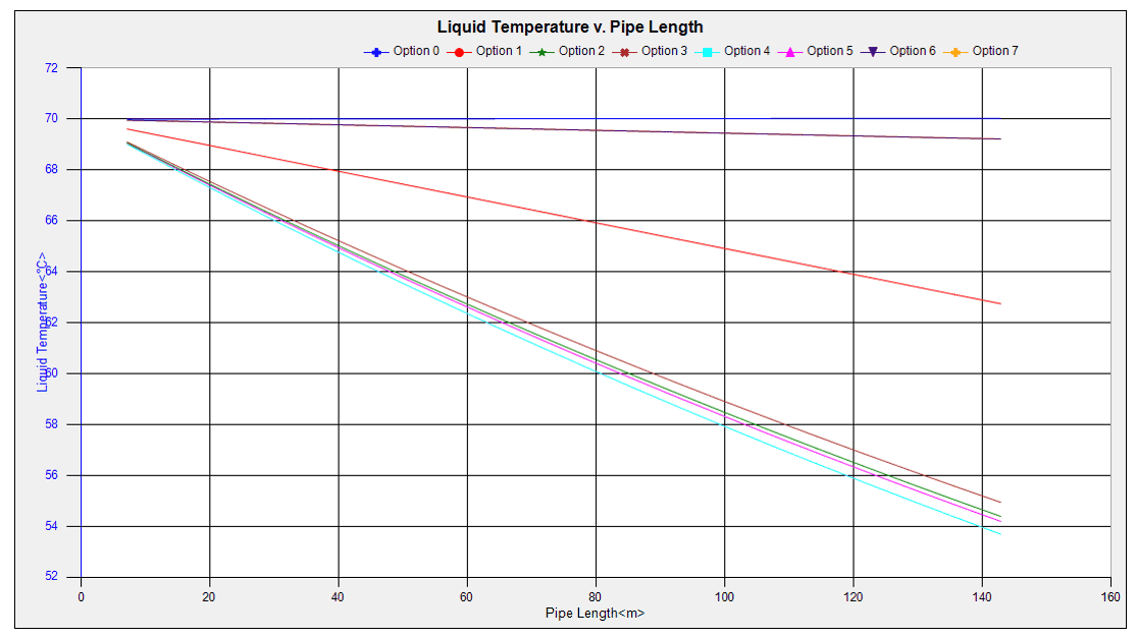
For option 0 (adiabatic) no heat rejection is considered, there is however a slight heat increase due to friction.
For options 1 and 2, no heat transfer is modeled between the fluid and the pipe, nor between the pipe’s inner and outer walls. As a result, the liquid temperature is equal to both the interior and exterior wall temperatures. Additionally, in option 2, the heat transfer area is based on the total external surface exposed to the ambient environment, calculated using the diameter of both pipe insulation thickness.
In option 3, heat transfer between the liquid and the interior pipe wall is modeled using the Dittus–Boelter correlation. Thermal conduction through the pipe material is neglected leading to the same temperature for the interior and external wall, but not the same as the liquid temperature.
In options 4 and 6, heat transfer is modeled between the ambient environment and the outer pipe wall, as well as, thermal conduction between inner and outer walls, but not between the fluid and the pipe. As a result, the liquid temperature is equal to the interior wall temperature, while the exterior wall temperature is different.
For options 5 and 7, the complete heat transfer process is modeled, including heat transfer from the fluid to the inner wall, through the pipe wall to the outer wall, and from the outer wall to the surroundings. Therefore, the fluid, interior wall, and exterior wall temperatures are all different.
Lastly, the effect of burying pipes was investigated. The comparison between a well insulated pipe and a fully buried pipe provided similar results in this study with only minor heat loss for the simulated 150 [m] of pipe. The difference is more drastic when comparing these with a fully exposed pipe.
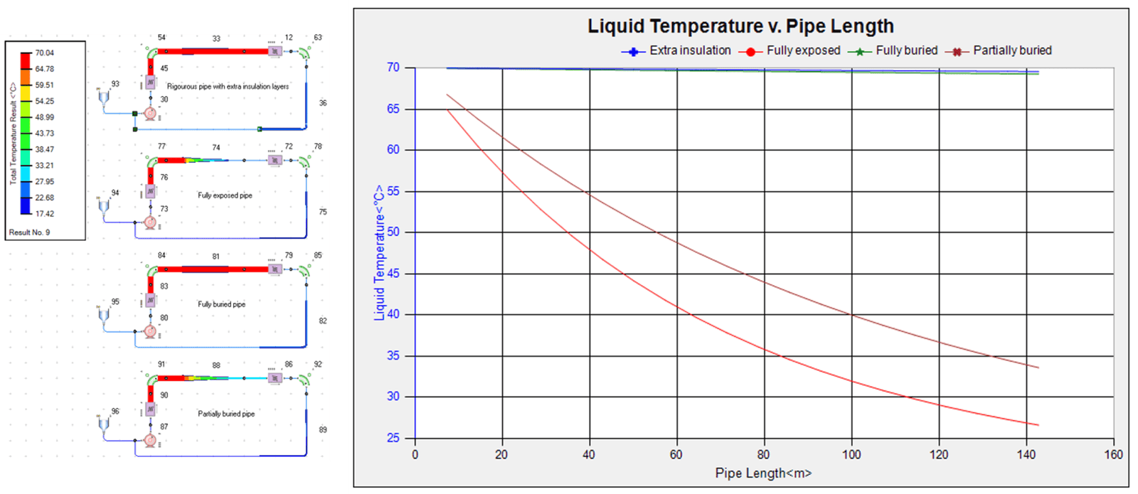
Variation of temperature for insulated, buried and exposed pipes
We hope you have found this article interesting. If you have any questions or comments, please feel free to reach out to us at support@volupe.com.
Author
Fabian Hasselby, M.sc.