In this week’s blog post we will take a closer look at the SPH (Smoothed Particle Hydrodynamics) solver in Simcenter STAR-CCM+. As part of the multiphase capabilities the SPH solver was introduced to Simcenter STAR-CCM+ in its most rudimentary state in version 2402. We will summarize its capabilities over the different versions since release, and we will take a look at a test case and see how to work with the SPH-solver. What setups to do, mainly focusing on how the workflow might differ from what we are used to with the volume mesh based, finite volume method we all know and love.
History in Simcenter STAR-CCM+
2402 – Introduction of the SPH solver into the main GUI of Simcenter STAR-CCM+. It also come in its initial state with a speed-up of about 30% compared to SPH Flow, the software that Siemens acquired a couple of years back.
2406 – Introduced the inlet boundary condition, from here it was possible to have a jet of liquid injected into the domain. Also added report for removed particles.
2410 – Surface tension modelling was introduced as part of the multiphase interaction. A stabilization option enhancement was also introduced to help stabilize the free surface. Full parallelization of the initialization was added. A Single GPU-native solver was introduced.
2502 – The boundary integral method was added to better handle particle-wall interactions and allow for more complex geometries including sharp angles. Multi-GPU acceleration was introduced.
How does the SPH-solver work?
The SPH method is a type of Lagrangian formulation that does not need to take into account the finite volume approach, while still being based on the Navier-Stokes equations. It was initially developed for astrophysical problems and was later adapted to be suitable for free surface flows. Instead of using a finite volume approach, the fluid is discretized into dynamic elementary points, referred to as particles, without predefined connectivity. An important concept for SPH is the kernel (smoothing) function that considers the influence of neighboring particles on one another with a specified radius. Different from the volume mesh-based methods that require explicit tracking of the interface between two phases, the SPH directly simulates a free surface for interactions between two-phase-fluids. A zero pressure is enforced at the free surface due to the absence of particles in the gas phase, eliminating the need for explicit surface definition. The particles represent the higher density fluid, and the lower density fluid is represented by the non-discretized space. It is important to remember that the SPH-method is an incompressible method, both for the liquid phase and the gas phase.
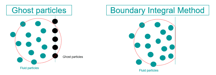
There are two different methods of handling wall interactions as of version 2502 of Simcenter STAR-CCM+. The first one is the Ghost Particles method. In this method we let ghost particles interact with fluid particles and enforce the boundary condition by extending the fluid domain up to the wall and apply appropriate fields to satisfy the condition. The SPH kernel is not truncated near the solid walls, so this is then achieved by introducing ghost particles on the wall for the particles to interact with, instead of directly interacting with the wall. In practice the surface-based term is reformulated as an integral over a ghost volume. In the other method, the BIM (Boundary integral method) particles instead interact directly with the wall, by interacting with the surface integral of the wall. Meaning that the surface-based term of the particle interaction is an actual surface based term, and does not use a volumetric formulation like the ghost particles method. The picture below gives a pictographic idea of the difference between the methods.
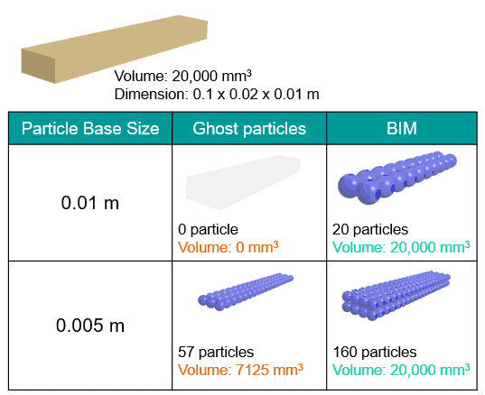
The ghost particle method has issues when it comes to describing complex geometries as it is necessary to form a volume representation of ghost particles to describe the surface. The picture below can show the issues we can get around by using the BIM method instead of the ghost particles method. We use a volume as an example, and the ghost particle method at a coarse discretization, will not fill the volume and respect the correct volume of fluid. Using BIM instead, even at coarse discretization, you will always respect the correct volume. In practice the BIM method can get better accuracy, even at a coarser discretization. It is therefore the recommended model to use.
There are a couple of options for the kernel formulation, Cubic and Wedland, where the latter is recommended for more robustness. Both methods also allow for a “Higher order Boundary Integral option” that can be disabled to increase simulation speed at the cost of accuracy. It is also possible for the BIM method (not the ghost particle method) to modify the kernel size. The size of the kernel is controlled by the ratio between kernel radius and particle diameter. A higher kernel size increases the number of neighbor particles which subsequentially lead to higher calculation cost. The recommended setting is between 2 and 3. Below 2 greatly affects the interpolation and above 3, the SPH interpolation is too high.
Another important aspect of using the SPH-solver in practice is the use of particle remediation. Similar to what can be done with the Lagrangian solver, where we remove particles that we select based on certain criteria, and we have the option to do this for SPH as well. This is used to remove particles from the simulation to optimize computational resources and ensure robustness of the solver. There are three methods for this using the SPH solver, we can remove particles based on position, simply particles that fall outside of the domain, pressure or velocity. Particles with too high pressure or velocity are then removed. For the BIM method it is recommended to use the pressure and velocity remediation to improve stability.
There is also a shifting method that helps maintain a homogenous particle distribution. It corrects particle location to give higher accuracy. It essentially moves (shift) particles to fill holes where holes should not form.
How to work with the SPH solver?
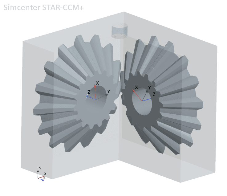
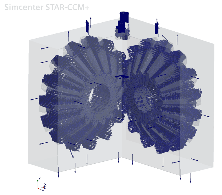
Now that we have had some insight into the workings of the SPH-method (actual equations can be found in the documentation) it is good to go over how we set up a simulation using the method. We will focus on the main differences between the workflow for the SPH-solver and a simulation using the finite volume approach. We will use an example as base for that. In the example two angled gears are located and the domain around is shown. We also have an inlet at the top for the liquid phase. The liquid that enters is a generic oil. Note also the added custom coordinate systems that will be the basis for each gear’s rotation in the simulation. It should be noted that rotation can be specified in the frame of a cartesian coordinate system (not in a cylindrical coordinate system). Based on the method used you should consider the resolution of your objects. In this example the gears are surface wrapped, and the rest uses the tessellation from shape parts that has been subjected to a number of Boolean operations to create the desired shape.
The next step after creating the geometry is to assign parts to regions, similar to what we do for a mesh-based simulation we “Assign parts to regions”. And when we do that, we do not require a fully subtracted volume, and what do I mean by that? From the previous picture we see that our domain will consist of three parts, the two gears and the surrounding geometry. We do not require that our gears have representation or inheritance in the surrounding part, but we instead select separately for our three parts their representation. We do however, leave the default of creating one region for all parts together with a surface topology, and we select the option of creating a boundary for each part surface. This will create a surface topology where we, in one region, have all our individual parts, including the gears, as separate surfaces. Once we have assigned the parts to our region, we need to use the expert property of “Allow Per-Part values”. That option lets us treat the different surfaces in our region based on part-input. In our example it is necessary to set the gears as separate sub-groups while the rest of the surfaces can remain in the default sub-group.
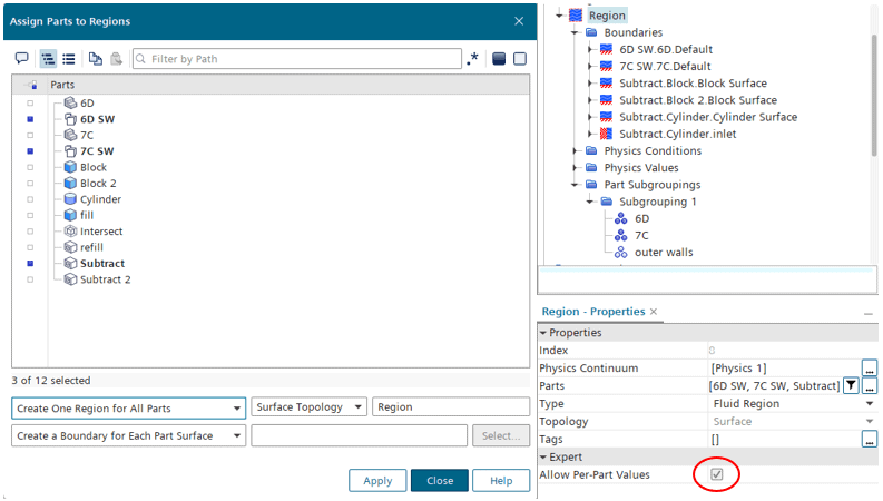
But why is this important? For two reasons mainly, motion and orientation. The sub-groups are defined under the region, in the Part Subgroupings, there you create additional subgroups and assign the relevant parts. Note, that the particle base size is set under region physics values as well, there is no injector specification as we would have for the Lagrangian solver, but the particle size is set directly on the region, and is comparable to the mesh size. So far, using the SPH-solver, the particle size is constant in the entire region. Rotation is set for each part subgroup under Direct Rotating Motion values. You can set motion based on a custom coordinate system that is cartesian, but not a cylindrical one. Under part orientation you can reverse the orientation of the parts. Particle generation allows you to specify the domain or subdomain where particles are initialized, basically the liquid level. Remember however that the part selection of particle generation needs to be an exact subdomain of the intended calculation domain. That part cannot extend beyond the domain nor can it cover the inside of the gears in this example or particles will be initialized there. Utilize the Boolean subtract operation to create the correct subdomain.
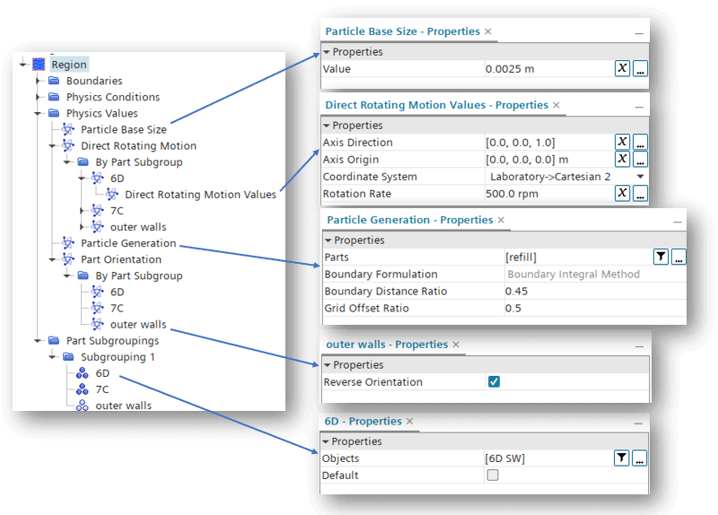
The reason why part orientation is important is that the particle interaction with the walls can only happen on the “back-side” of surfaces. Meaning that to interact with a particle, the normal of the surface must point away from the side where the particles reside. The picture below shows the necessary orientation for our surfaces for particles to stay in the domain. The normal on the outer walls need to point outwards wards since it is the inside we want interacting with the particles. And if this does not correspond initially, you can utilize the reverse orientation on separate sub-groups to make sure your calculation domain is set up correctly.
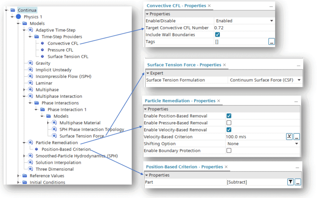
For the model selection using the SPH solver there are some things which are good to keep track of. The SPH-solver is recommended to be used together with Adaptive Time-Step. There are five timestep providers available, Convective CFL, Pressure CFL, Surface tension CFL, gravity CFL and Viscous CFL. You are recommended to use all of them when using the explicit solver and all but the Viscous CFL for the Implicit solver.
There are two formulations for the Surface tension, the first option is the Continuum Surface Force (CSF), a simpler description useful where the curvature of the interface influences the dynamic of the fluid flow. The other option is the Continuum Surface Stress (CSS), an effective option for simulations where surface stress varies directionally or where anisotropy in surface tension is significant. It provides a detailed representation of the interface and is suitable for complex geometries, particularly sharp corners.
The particle remediation option has been mentioned, where we simply exclude particles based on certain conditions. The position-based removal lets you select a shape, that shape is then applied using a bounding box, to exclude what falls outside. For the velocity-based option you remove particles that reach above a certain velocity and the pressure-based remove above a certain pressure value.
Once you have selected your models, set the properties of your liquid, defined your time-step providers, selected the remediations to include and set your boundary conditions, you are set to run your simulation. Below is animation of what it can look like using our example. The plot shows the timestep selected by the adaptive timestep provider for each subsequent timestep.
I hope this has been useful in understanding both how the SPH-solver works and how to actually work with it. The SPH-solver requires an additional license increment to your license file. Contact your Volupe sales representative for a quotation. Remember to reach out to support@volupe.com with any questions.
Author

Robin Victor
+46731473121
support@volupe.com