In this week’s blog post we will investigate Lagrangian post-processing and more specifically the function of boundary sampling. We will use it to track particles hitting a wall with a stick boundary condition and give an example of how to analyze data on these particles.
Setting up the boundary sampling
Boundary sampling is a way of tracking Lagrangian parcels and their interaction with specific boundaries and can be used as an alternative to using track files. Contrary to using track files (which are used to store your particle tracks in standalone files) the boundary sampling function allows you to monitor the progression of particle properties as your simulation is running without having to save the simulation or loading track files. This of course allocates additional memory, so it is recommended to use this function with caution for cases with a large number of particles. It is important to know that the boundary sampling method only stores the last Lagrangian step, which means that you must monitor your values of interest to see the historical progression. Also, since boundary sampling stores data only locally, it cannot be used to display trajectories.
To set up a case using boundary sampling, simply move into your Lagrangian Multiphase Models selection and tick the box for boundary sampling.
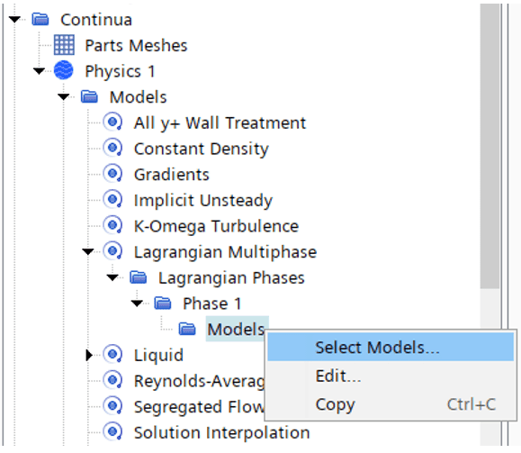
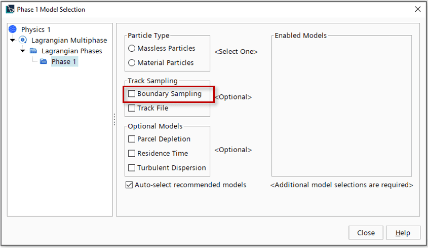
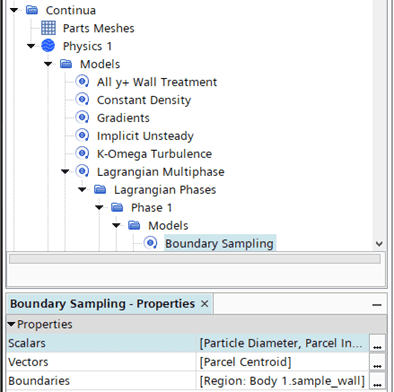
Once selected, a Boundary Sampling node appears under the Lagrangian Multiphase Models folder. This is where you specify the Scalar and/or Vector field functions that you want to sample and also the boundaries where you want to store your data. In this case we want to analyze the diameter distribution of particles hitting a stick boundary. Some properties are selected by default, such as Parcel Index, Particle Count and Time, but in addition to these we now also want to select the scalar “Particle Diameter”. In this case we want to sample this particle data on a boundary called “sample_wall” which is part of our “Body 1” region. Now we are done setting up the boundary sampling.
Analyzing particles on stick boundaries
A challenge with the stick boundary condition is that it terminates the parcels interacting with the boundary, meaning you are no longer able to evaluate or visualize properties on these parcels. There is however a workaround for this which we will explain in below.
The method is based on an injector type functionality built in to Simcenter STAR-CCM+ called “Parcel Transfer Injector”. The conceptual idea behind the method is to transfer all parcels sticking to our sample boundary into a post-processing phase using a stick criterion.
Parcel transfer methodology:
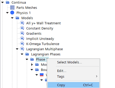
- Copy the Lagrangian phase your tracking and paste a new identical one into the physics continua. Give the new phase a suitable name, e.g. “evaluation”.

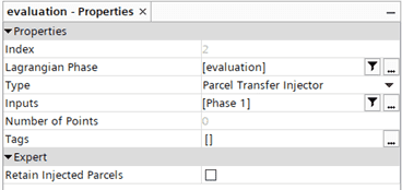
- Create a new injector. Pick “evaluation” as the Lagrangian phase and “Parcel Transfer Injector” as Type. Pick your main Lagrangian phase as Input. What we do here is basically telling STAR-CCM+ that what we introduce (or inject) into our evaluation phase is based on output from “Phase 1”.

- Under “Injector > Injector name > Values > Transfer Criterion” go into the editor and type ${StuckMark} (see picture below). This is a reference to the field function “Parcel Stuck Mark” which is an indicator whether a Lagrangian parcel is stuck (1) or not (0) on a stick boundary. This means all parcels in the main Lagrangian phase that get stuck on your stick boundary will be transferred into this secondary Lagrangian phase (called evaluation).

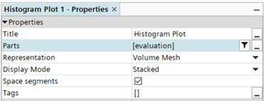
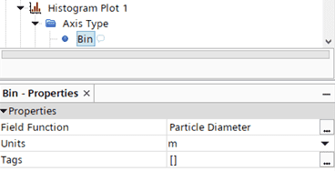
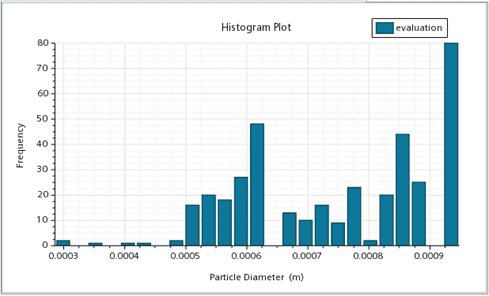
- Now you can use the “evaluation” phase to post-process and analyze the particles that have stuck on your sampling boundary. Below is an example of how you could use a histogram plot to look at the particle diameter distribution.


Using this methodology you can of course also play around with e.g. derived parts, such as thresholds, to analyze specific parts of your transferred data.
We at Volupe hope this blog post was helpful to show how you can work with boundary sampling and stick boundaries. If you have any questions or comments you are always welcome to send them in to support@volupe.com.
Author

Johan Bernander, M.Sc.
support@volupe.com
+46 702 95 18 31
