Automation of repetitive tasks is the best! I personally enjoy every task that could be automated. And that is why I admire Simcenter STAR-CCM+ so much. STAR-CCM+ is developed from ground with the intention to bringing all the stages of the virtual prototyping process into one platform. In doing so we find several functionalities to completely automated the workflow. Backbone to this is a pipelined process which is replay-able with just a couple of clicks. In this week’s blog I focus a marine application and show the options you find in Simcenter STAR-CCM+ to automate a series of simulation runs to generate a propeller open water curve.
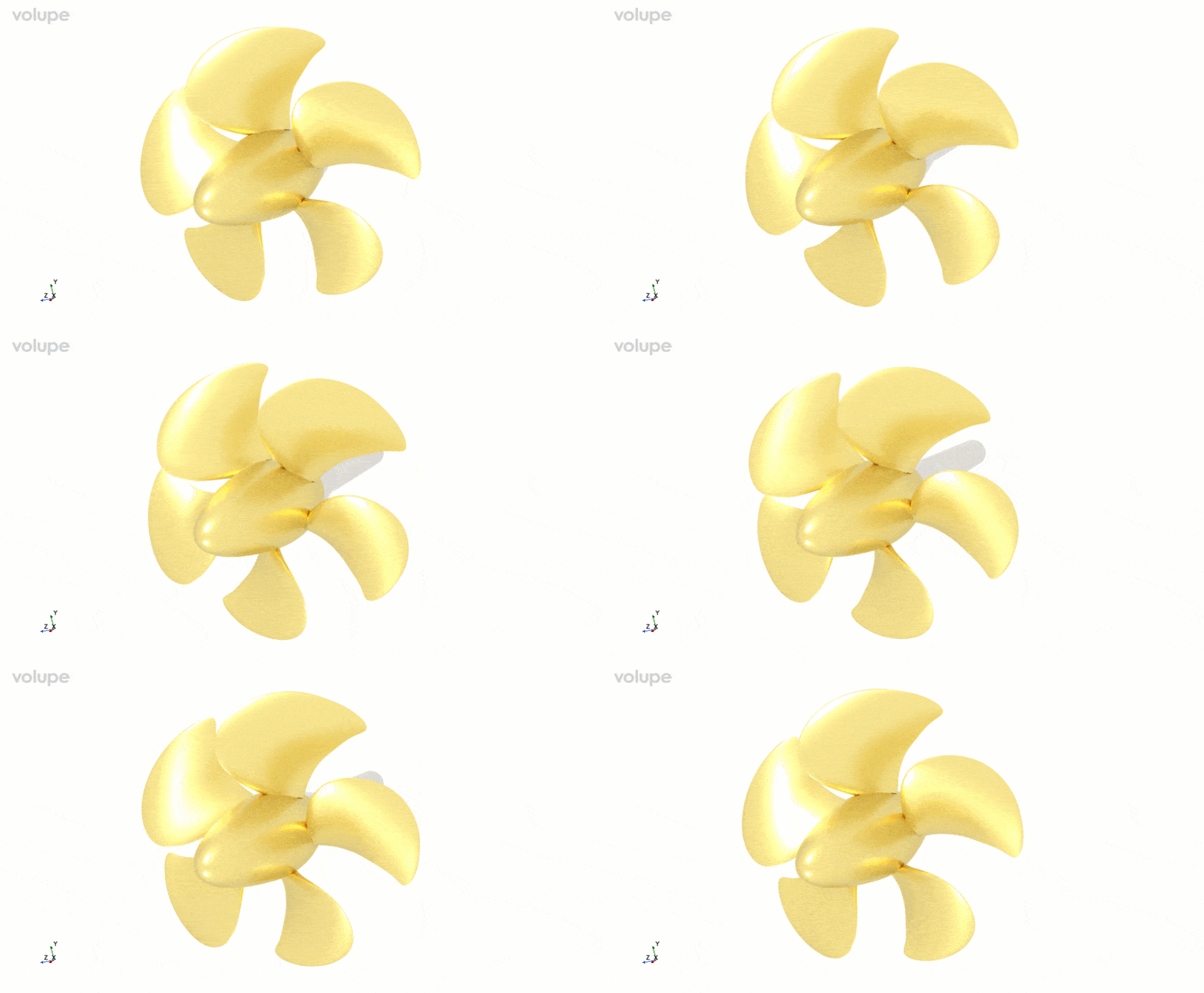
The simulations shown here are based on the “Moving Reference Frames: Marine Propeller in Open Water” tutorial which demonstrates the workflow for setting up an open water simulation for a marine propeller. The geometry is the Potsdam Propeller Test Case (PPTC). Open water characteristics of propellers are carried out to measure the characteristics in a homogeneous inflow by varying the inflow velocity. This requires however, a series of tests or simulations.
In Simcenter STAR-CCM+ you can automate such series in different ways by using:
- Design Manager
- Simulation Operation
- Java scripting
Here we will focus on the Design Manger setup and the Simulation Operation usage. However, the latter one can conveniently be combined with java scripting for propeller simulation to switch between steady and unsteady simulations.
Design Manager
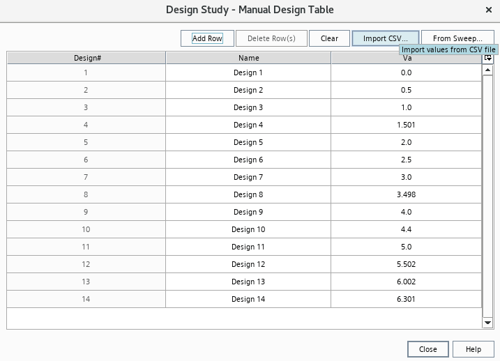
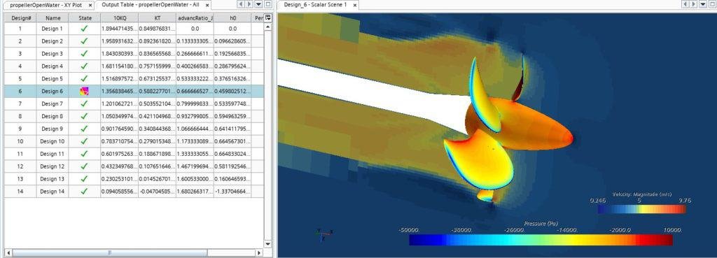
Once you set up your baseline simulation of a single inflow speed, you can create a Design Manager project out of the simulation file. In our case for the open water curve, we want to calculate a specific set of inflow velocities according to the measurement at SVA Potsdam. So, we create a manual design Study and import the velocities from a csv file.
With the build in functionality in Design Manager, we can easily create a plots and snapshots to evaluate the obtained results at each inflow velocity.
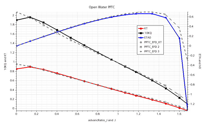
The results are saved after the Design Study has finished and can be accessed for further post processing, or detailed analysis. We also have several options for distributing the simulations on a cluster to your best applicability.
Simulation Operation steady state
However, sometimes you need a bit more flexibility and simplicity. In that case simulation operation can be applied in stead of creating a Design Manager project. One example can for instance be in case you want to run simulation in batch mode with automated I/O operation.
In case of the Propeller Open Water analysis we can combine Simulation Operation with Java scripting to read a text file which contains the velocities and to write propeller coefficients to a csv, to automate a batch simulation. So far it is not possible to natively run Java macros from a Simulation Operations tree. But a workaround is to use overarching macro that runs the simulation and checks the Simulation Operation tree for macro execution commands as described here.
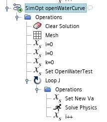
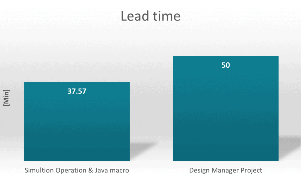
This way we can read in the velocities into an array inside the driving java macro and create a Simulation Operation that loops through the velocities. Such a setup is beneficial since we start the new velocity run from the previous velocity and can gain better convergence. In fact, the Simulation Operation went through the states 1.3 times fast only because of the reduced overhead for file manipulation.
To use the macro, just insert a Set Parameter operation in the Simulation Operation pipeline at the point at which you want your macro or function to be executed. The operation “Set New Va” will for instance trigger the following action:
- Get the current index of velocities
- Update the simulation parameter “Va”
if (blockName.startsWith("Set New Va")) {
   int vaIndex = (int) parameterI.getQuantity().getValue();
   parameterVa.getQuantity().setValue(VaList.get(vaIndex));
   sim.println("New Va = " +  VaList.get(vaIndex));
   sim.println("New J  = " +  parameterJ.getQuantity().getValue());
}
To update the plots only at an update of J, increment of the loop counter triggers an Update Event. The method is described here (Using Simulation Operations for parametric sweep) and can also be used to save the simulation state to a simulation history file.
The simulation operation Set Parameter “i++” increments the loop counter and triggers the generation of output data:
if (blockName.startsWith("i++")) {
   int jIndex = (int) parameterI.getQuantity().getValue();
   Report  Report_J   = sim.getReportManager().getReport("advancRatio_J");
   Report  Report_KT  = sim.getReportManager().getReport("KT");
   Report  Report_KQ  = sim.getReportManager().getReport("10KQ");
   Report  Report_ETA = sim.getReportManager().getReport("h0");
   J[jIndex]   = Report_J.getReportMonitorValue();
   KT[jIndex]  = Report_KT.getReportMonitorValue();
   KQ[jIndex]  = Report_KQ.getReportMonitorValue();
   ETA[jIndex] = Report_ETA.getReportMonitorValue();
}
To update the plots only at an update of J, increment of the loop counter triggers an Update Event. The method is described here (Using Simulation Operations for parametric sweep) and can also be used to save the simulation state to a simulation history file.
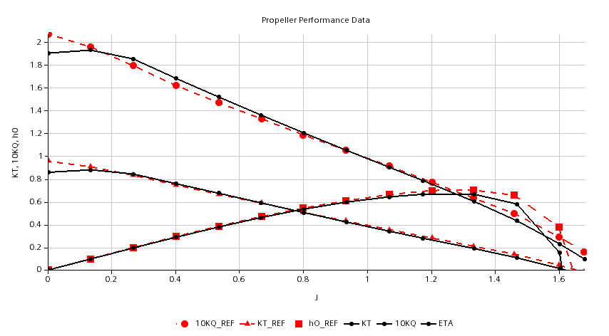
In the end we update the performance plot by reading the newly written csv file into a table to plot the result together with the experimental data:
// Update the plot with calculated propeller characteristics
Table fileTable_1 = sim.getTableManager().getTable("propellerPerformanceData");
fileTable_1.extract();
Simulation Operation steady-unsteady mix
This sounds like a lot of workarounds to get something which is very straightforward using the Design Manager. So, is it worth it? Maybe not if you do an open water curve only. Because open water curve simulation is done for homogeneous inflow which can be simulated perfectly with a MRF approach in a steady simulation. But in case of a simulation in behind condition?! Such simulation would require switching from your steady simulation to a transient simulation after the flow developed. And then you will need to gradually reduce the time step get a sufficient temporal discretization. Now, the actual advantage comes into account, combining Java scripting with Simulation operation. Because in this case we can extend the velocity loop with an unsteady simulation where we loop again to stepwise reduce the time step length automatically.
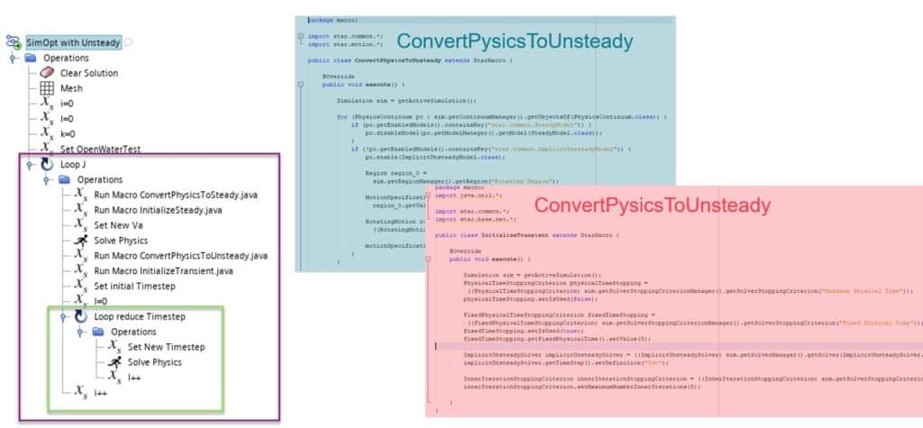
To switch between steady and unsteady physics, we split the macros into elementary functionalities, such that each macro is very short and easy to read and maintain (possibly extending with some additional automation like changing the annotation).
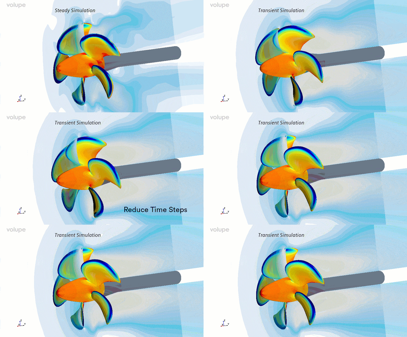
The unsteady simulation of the propeller will be initialized with a temporal discretization of 8 degrees rotation per time step. During the second loop this will be reduced stepwise to 1 degree before the velocity is updated and the simulation switched back to steady state again.
I hope that this has been useful and a way to give you some insight to the tools available for you as a STAR-CCM+ user. If you have any questions or are interested in the files used for this case, as usual, reach out to us at support@volupe.com.
