In many engineering simulations it can be beneficial to utilize symmetry or periodicity to reduce model size and complexity. But for post-processing purposes, it is often helpful to visualize the full geometry. In Simcenter STAR-CCM+ you can achieve this using idealizations or transforms. This week’s blog post will outline how and when to use these features for post-processing.
The concepts of idealization and transform
In many cases, the concepts of idealization and transform can be used to achieve the same visual representation. But fundamentally, they differ a bit in terms of definition.
An idealization in Simcenter STAR-CCM+ refers to the process of simplifying a simulation to reduce the computational effort, while maintaining an accurate representation of the geometry. This can be achieved by utilizing e.g. symmetry or periodicity, meaning that an idealization is not really a method or an operation in itself, but rather a tool that becomes accessible to account for the simplifications that you have made.
A transform in Simcenter STAR-CCM+ refers to a mathematical operation that can be used to modify e.g. a position, orientation or shape of an entity. As such, transforms can be used to move, rotate, scale or reflect geometries, as well as to create complex motions or deformations.
Now let’s exemplify how to utilize these concepts for post-processing.
Presenting the full domain
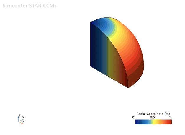
We will use an example to show how you can make use of the concepts described above. Let’s assume we have a geometry in the shape of a sphere. We then decide that we can utilize symmetry to reduce our domain to 1/8 of a sphere to save some computational effort. We end up with a domain as shown below.
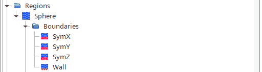
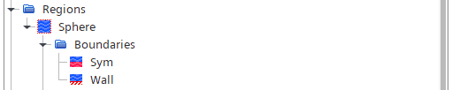
In this case we have four boundaries:
- Symmetry in the X-plane
- Symmetry in the Y-plane
- Symmetry in the Z-plane
- The sphere’s outer face.
As a result from the boundary setup that we’ve made (i.e. using symmetry conditions) the Tools -> Idealizations folder is now populated with a so-called symmetry idealization (see below).
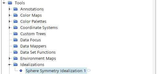
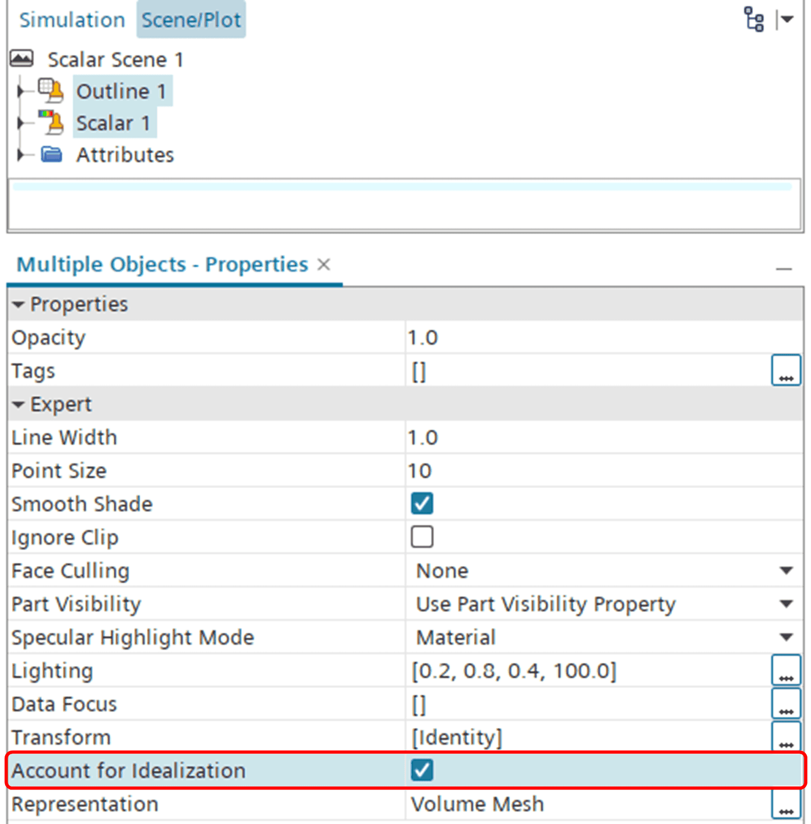
This Idealization is now ready to be used to visualize the entire sphere in a scene. To do so, you simply tick the box “Account for Idealization” for each displayer that you want to include.
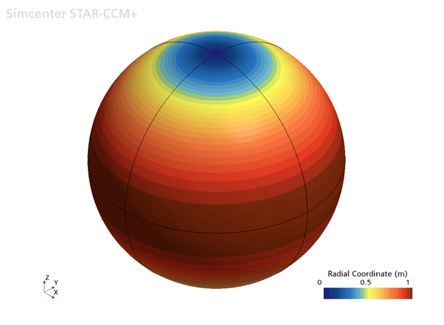
In this particular example, the scene will now look like this:
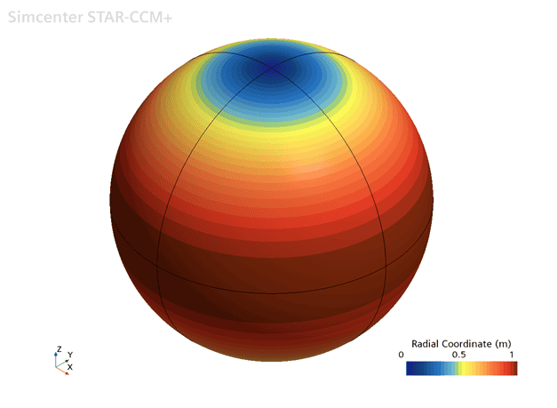
So, using the predefined symmetry idealization, we can effectively visualize and plot physical properties on the complete geometry, even though we have simulated only 1/8 of the domain. As described in an earlier blog post about axisymmetry, idealizations can also be useful for e.g. reporting values for cases with symmetry or periodicity (Axial Symmetry In Simcenter STAR-CCM+ – Volupe.com).
Now, let’s assume that the case was set up a bit differently, with only one single symmetry boundary instead (a completely valid setup, and in all fairness an even more efficient one). We would then have two boundaries instead:
- A symmetry boundary (including SymX, SymY and SymZ faces)
- The sphere’s outer face.
For this type of setup, the idealization would not work, as STAR-CCM+ would not understand how to treat the different face normals in the input to the symmetry boundary. The “Account for Idealization” option would hence have no effect.
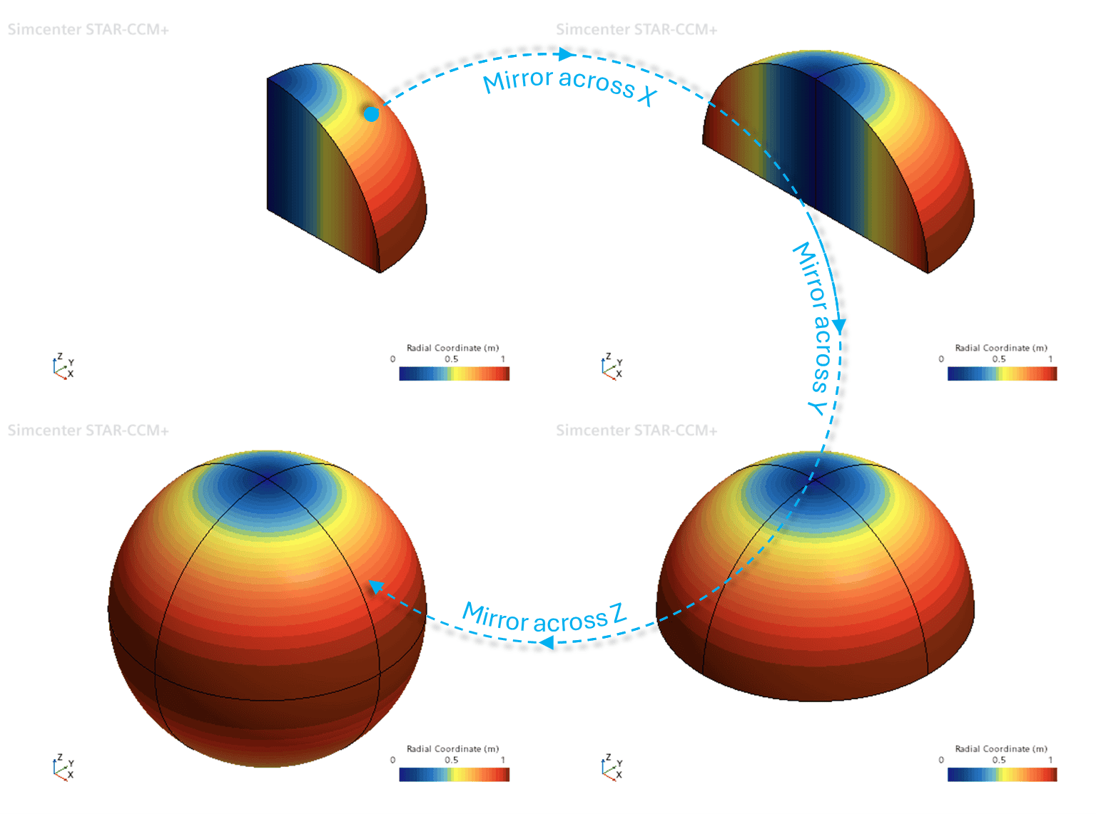
So how could we overcome this if we chose this setup from the beginning? You probably guessed it – we could use Transforms. And more specifically, we would have to use so-called Superposing Transforms. You can think of it as unfolding a napkin. We mirror our displayer once across the X-plane, then across the Y-plane and lastly across the Z-plane. Then we end up with a full representation of the sphere. The “sequence” is also exemplified below. Note that you don’t have to perform the actual sequence within the scene – the picture is simply an explanation of what is done within the Superposing Transforms.
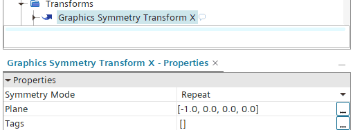
So, let’s take a look at the steps you need to take to set up the Transforms. We start by right-clicking the folder Tools -> Transforms and select New Graphics Transform -> Graphics Symmetry Transform.

The input needed for the Graphics Symmetry Transform is the symmetry plane’s normal axis and the plane coordinate in the normal direction, i.e. [X, Y, Z, Coordinate]. As mentioned above, we want to start with mirroring across the X-plane. In this case our reference, or so-called “Identity” geometry, lies within the first octant, so we want to start with mirroring in the negative X-direction at coordinate 0, i.e. [-1.0, 0.0, 0.0, 0.0] as depicted below.
To establish the full “unfolding sequence” of the sphere we now make use of the Superposing Transform. As we expand any Graphics Symmetry Transform node, we can see there is a folder for Superposing Transforms.

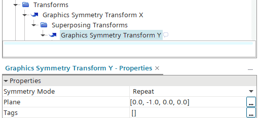
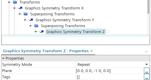
As depicted above, we create a sequence of Superposing Transforms to include the previous Transform in the downstream Transform. As described earlier, in this case we want to mirror around the X-plane, then the Y-plane and lastly the Z-plane. This requires the following input to the Graphics Symmetry Transform Y and Graphics Symmetry Transform Z:
Finally, we move into our scene to make use of the transform to visualize the full sphere.
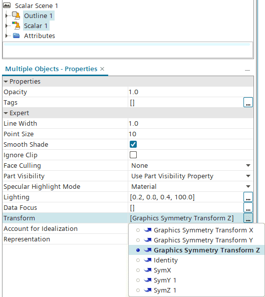
We then end up with a depiction of the entire sphere in our scene, similar to before when using the idealization.
I hope this blog post has been useful to show how you can use built-in functionality to improve post-processing when you’re using e.g. symmetry or periodicity. As a final note, it is worth mentioning that these features require a volume mesh representation to work.
Author

Johan Bernander, M.Sc.