It this week’s blog post I would like to cast some light on some of the more abstract concepts when talking about multiphase simulations, especially in the Eulerian framework. I will go over the concept of phase interaction topology, how that impacts your multiphase simulation, depending on your flow regimes, and the type of physics you are trying to solve. Consider this post a deep dive into some of the concepts introduced in the post [Multiphase modeling capabilities in Simcenter STAR-CCM+ – VOLUPE Software].
Further I will explain Interaction area length scale and Interaction area density, and why these concepts are paramount to your Eulerian simulation.
All these concepts are good to understand. Understanding these can help you when something in your simulation is wrong. Once you have tinkered with the values for all constants in your sub-models and your simulation still diverge, you can start considering if the interaction between your phases makes sense (or do that from the start). Hopefully this will be clear once you have read the following sections.
The reason why these concepts are important in a Eulerian simulation is because different phases are not explicitly modelled. Except for simulations where interfaces are tracked or captured, like VOF or LSI-simulations, but these are special cases. Imagine bubbles rising in a column of water (the example of Hibiki’s bubble column, a tutorial described in the Simcenter STAR-CCM+ documentation). What you have is a rather simple case with bubbles of constant diameter entering the domain (figure of the example, in the left part of the picture below). Using a population balance to describe the bubbles interacting with the continuous flow and each other, you will typically evaluate your bubbles as shown in the right picture below. Meaning that there are no actual bubbles to be found, you cannot single out any individual bubbles in your domain, even though you have complete control over how many you send into the pipe. You will instead look at the Sautern mean diameter (the right picture in the figure below). Your model selection has used a number of closure models, in this case e.g. for collisions, coalescence, virtual mass, drag force, lift force etc. And the closure models for these sub-models are all directly or indirectly impacted on what settings you have for Interaction area density.

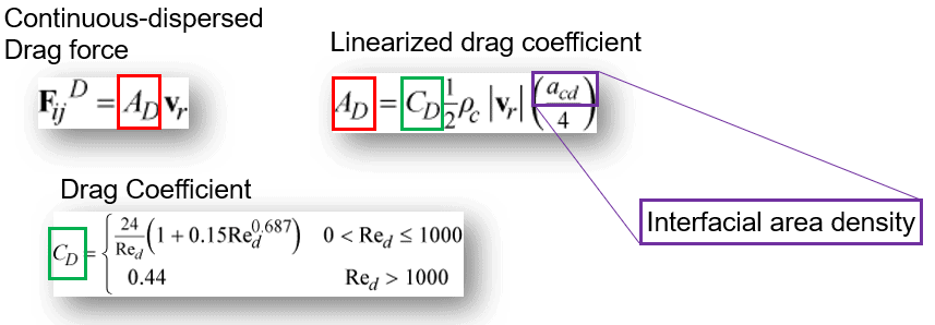
In the picture below are some of the relations for the commonly used Drag Force calculation. These equations are used if you include drag force, when simulating some sort of bubbles, droplets, or particles. The force acting on phase i based on the drag of phase j is described as the first equation for continuous-dispersed drag force. Part of the linearized drag coefficient expression (equation to the upper right) is the Drag Coefficient (the bottom equation), but also the value for the Interfacial area density. A common model for Drag coefficient is the Shiller and Neuman model, used in the example. But what about the value for interfacial area density? The interfacial area density is specifying the interfacial area available for momentum, heat, and mass transfer exchange between phases. It does not matter how correct your closure models are, the simulation will not be correct, if they are used with the wrong values for area interacting. My point is that the concepts is part of most closure models and are specified by the user. That is why it might be good to understand them as such, and that is the reason for this blog post.
Phase Interaction topology
Your phase interaction topology is based on the type of problem you wish to resolve. In Simcenter STAR-CCM+ you do not initially select phase interaction topology, but rather your model selection for your physical phenomena decides what phase interaction topology will be available to include. Let me give an example:
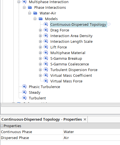
The Hibiki bubble column described in the previous section. The selection of particle size distribution in the physics continua makes this into a Continuous-Dispersed Topology simulation. That selection provides the information that the air entering as a dispersed phase into the simulation, and that can be seen in the properties of the model in the phase interaction.
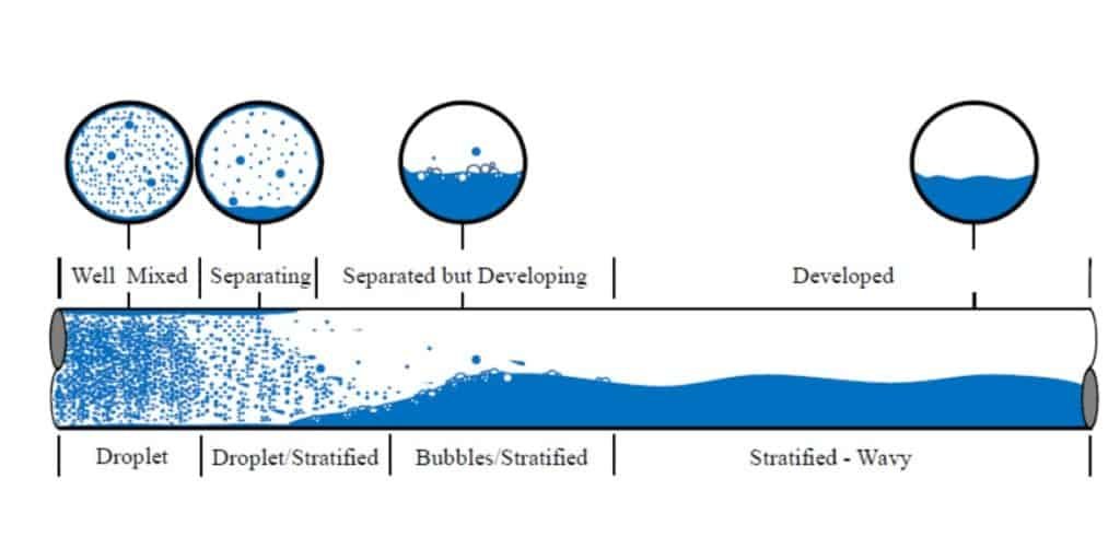
The previous example uses the continuous-dispersed topology. It is then enough to use one interaction. But what if my simulation span over multiple Flow regimes? And what if it needs an interaction topology that can describe, for instance, both continuous-dispersed and stratified flows, like in the picture below. Or even flow that varies which phase is the dispersed one and the continuous one.
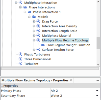
In a simulation describing a system like this, we need both a separate two-phase flow and a dispersed phase in either of the two (or both) stratified phases. This is done automatically in Simcenter STAR-CCM+ by employing a volume fraction-based criterion to classify the flow regime into dispersed and separate two-phase flows. Instead of the continuous-dispersed topology, the Multiple flow regime sets a primary and secondary phase. From that, three flow regimes can be defined:
- The secondary phase is dispersed in the primary phase
- An interface regime where both phases are separated (e.g. stratified flow)
- The primary phase is dispersed in the secondary phase.
As stipulated in the example case with Hibiki’s bubble column, since none of the regimes are explicitly modelled (again, unless you have interface tracking like LSI), an implicit way of describing these regimes are required. This is done using a weight function. Let’s not get too technical here and instead leave that for a separate blog post. Let’s say this, there are several weight functions to weight the impact that the flow regime has on the linearized drag and the heat transfer coefficient describing the interaction. These can be studied in detail in the documentation.
Interaction length scale
Interaction length scale describes the interaction between flow regimes. Simple as that! For your typical continuous-dispersed flow, think bubbles in water. The interaction length scale is the size of the bubbles, their diameter, but again since we don’t explicitly model the bubbles, we are forced to use a mean diameter value. Preferable is the Sautern mean diameter, defined as the diameter of a sphere that has the same volume/surface area ratio as the particle of interest.
Note that for particle size distributions calculation with the AMUSIG model you specify a number of groups, and these groups have their own separate Sautern mean diameters. You can read more about this in my previous blog post, regarding population balances [Population balance in Simcenter STAR-CCM+ – VOLUPE Software].
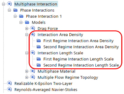
In a multiple flow regime simulation, you need to specify both the first and second regime’s interaction area densities and length scales.
Interaction area density
The interaction area density specifies the interfacial area available for momentum, heat, and mass transfer between each pair of phases in an interaction. As shown in the Hibiki boubble column example, the interaction area density is used directly. Simcenter STAR-CCM+ provides two models for interaction area density:

The spherical particle interaction area density model is based on the surface area of a spherical particle and is not applicable for high volume fractions. The symmetric particle area density is modified by the availability of the continuous phase and can be used for a wide range of volume fractions.
I hope this can give you deeper understanding of how to setup your Eulerian multiphase simulations, and what possibilities there are when doing so. Do not hesitate to reach out at support@volupe.com if you have any questions.
Author
Robin Victor
support@volupe.com
+46731473121
