This week we will take a look at the VOF solver, and more over the specific ways to use it to speed up your simulation. Over the last release of Simcenter STAR-CCM+ there has been a number of different updates and new models for the VOF solver. We hear things like Single-step, Multi-step, HRIC, MHRIC, Implicit VOF, explicit VOF. Even slip-velocity, that is usually more related to mixture modelling, is supposedly good for some situations using the VOF-solver. But what does it all mean? When do we use the models and what limitation does it pose to our simulations? Let’s see if we can explain the relevant concepts in this blog post.
The VOF solver
The VOF (Volume of Fluid) method is part of the Eulerian methodology, meaning that we look at a cell, and study all the inflows and outflows of matter, energy, and momentum to that cell. This is opposed to the Lagrangian methodology, where we instead follow a particle (or parcel) around in space. The VOF method is an interface capturing methods that predict distribution and the movement of the interface for immiscible phases. The method requires enough spatial resolution to resolve position and the shape of the interface between phases.
Distribution of phases and position of the interface are described by the fields of the volume fraction (referencing quadrant 1 in the picture below). The sum of all phases must sum up to unity (2) and depending on the presence of different phases or fluids in a cell can be distinguished (3). The distribution of the separate phases is driven by the mass conservation equation (4).

If there are two VOF phases present Simcenter STAR-CCM+ will only solve the volume fraction transport for the first phase. The value for the second phase is then simply 1 minus the value for the first one. When there are three or more phases, the volume fraction transport is solved for all phases and the value is normalized based on the sum of the volume fraction of all phases in each cell.
HRIC and MHRIC
HRIC is short for High Resolution Interface Capturing, and it is a scheme designed to mimic the convective transport of immiscible fluid components, which makes it well suited for tracking sharp interfaces. We will not go into the detail of the equations for the scheme, this can be studied in detail in the Simcenter STAR-CCM+ documentation. But know, that they are both based on the “normalized variable diagram” (NVD) that deals with convective transport. The HRIC has been around for a long time while the MHRIC (Modified HRIC) is a quite new addition to the software.
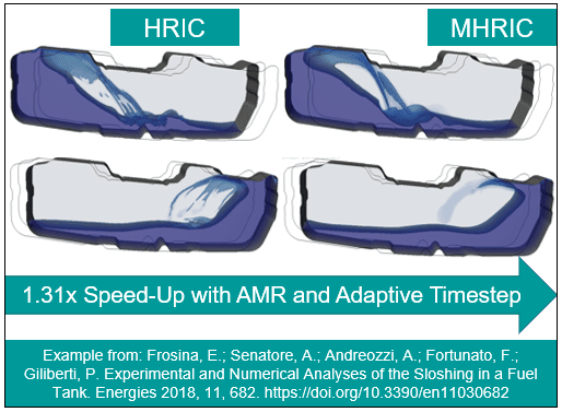
What is new and relevant here is the additions provided by the MHRIC. Many VOF simulations use AMR (adaptive mesh refinement) and adaptive timestep to get accurate results in a relevant timeframe. When using HRIC, this can lead to over-resolution for very small droplets and bubbles. In a large part of engineering problems, the smallest scales are not relevant to resolve to answer the engineering question, making the HRIC scheme represent unnecessary overhead. The MHRIC does not resolve the smallest features and consequentially leads to a reduced time to solution. The MHRIC also improved robustness and mass balance compared to HRIC and reduced the risk of artefacts at the free surface associated with e.g., the mesh. The MHRIC also produced a thicker interface, typically ~3 cells thick, without the interface leading to numerical mixture. The method provides a pragmatic approach to some engineering problems, like the example below with a sloshing tank, where each separate droplet and bubble might not be of interest.
Interface sharpening through temporal sub-cycling (Implicit/Explicit Single/Multi-step)
Using interface sharpening through temporal sub-cycling means allowing for some of the equations, the volume fraction equations, being solved aside, with a higher temporal discretization, from all other transport equations. If we start from the beginning and look at VOF single-step, that simply means solving the equation for volume fraction transport at the same time as other flow transport equations. Technically this is not temporal sub-cycling then since there is no temporal difference in when the transport equations are solved. This puts the demand that CFL<1 (or 0.5 for 2nd order time), or the free surface will be smeared.
On the other hand, we then have the VOF Multi-step solver, that then does the temporal discretization for the volume fraction transport equation. The multi-step solver then divides the full physical timestep into even smaller sections (N). This then allow the physical timestep to be selected independent of CFL-constraints. The methodology is supposed to always keep the interface sharp. The obvious downside of this is of course that it can result in unwanted levels of resolution and unnecessary overhead to our simulation time again.
Enter the Implicit multi-step method! Let’s first understand that the Explicit Multi-Step method is the default method. For explicit mult-stepping the number of sub-steps is decided by the other conditions, in this case the CFL-condition. The implicit option simply adds the possibility for the user to select the number of implicit sub-steps for the volume fraction solver. Where the Explicit solver decides automatically based on conditions, the Implicit solver lets the user decide. With this approach, the user can then indirectly discard smaller scale bubbles and droplets and this way allow for some levels of numerical dissipation. The table below describes the difference and briefly summarizes how the first-order time integrators work.

Note that the implicit method will not inherently work with any combination of global timestep and number of temporal sub-steps, but the volume fraction solution will (if the user is not careful) become increasingly diffusive. The two methods also differ slightly in how they are under relaxed, where the Explicit method applies the under relaxation after the last sub-step, the Implicit method instead imposes the under relaxation for each separate sub-step.
If you are interested in how the automatic determination of Sub-step Size in the Explicit Multi-step solver works, you are referred to the documentation.
Interface sharpening through Slip velocity modelling
You can add slip-velocity to the VOF method, and with this approach you will allow for a more physical behaviour of the multiphase scenario when the interface between the phase is not resolved. If you use this method, your VOF will behave more like MMP (What if VOF doesn´t work? MMP-LSI – VOLUPE Software).
In general, the VOF multiphase model assumes that the interface between phases is resolved. In Simcenter STAR-CCM+, near an interface, three cells exist; one where the volume fraction of phase i is 1, one where the volume fraction of phase i is 0, and one cell where the fraction of phase i is between 0 and 1. In the cell where the fraction is between 0 and 1 we have the interface, and the assumption that both phases move at the same velocity allows their motion to be described by a single velocity-field.
But, in some scenarios, where the requirement for VOF is not satisfied, to avoid the under resolved VOF behaving like a homogenous mixture with a smeared interface, we can include the slip between the phases. And this introduction leads to an improvement of modelling assumptions resulting in a recovery of a sharp interface.
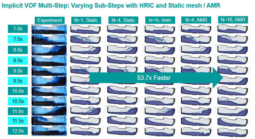
Comparing cases
Before releases of new features, they are of course tested and benchmarked. The picture below shows a 53 times speedup of an industrial case for a sloshing tank. Experimental data is compared to using the Implicit VOF multi step solver, varying the number of sub-steps, and varying between a static mesh and AMR.
Author

Robin Victor
+46731473121
support@volupe.com