In this week´s blog post we will work a bit more with post-processing, specifically the method of resampled volume. This relates to visualization and creating images to analyze. In a resampled volume we use a volumetric object to, in a semitransparent fashion, display scalar fields. Like looking at clip plane, or a surface, we can look at a volume field and evaluate our scalar field in a 3D setting. In this case we will look at a simple example with a sphere in a pipe. We will look at instant results from LES-simulation.

Simulation description

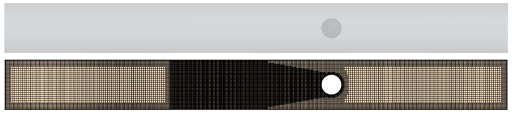
In the example we will use a pipe that is 1 m long with a radius of 5 cm, located with it center 35 cm from the inlet we have a sphere with a radius of 2 cm to obstruct the flow. The inlet velocity is 1 m/s. The bottom part of the picture also shows the mesh resolution of the case. We will focus our results inside the wake refinement (the area that is best resolved).

Creating a resampled volume

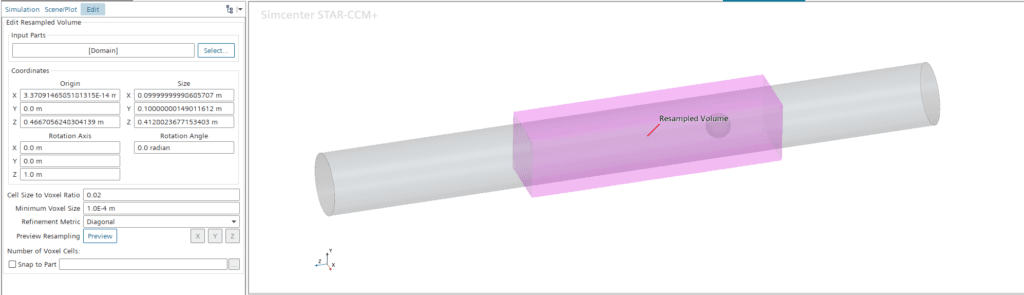
A resampled volume is created under derived parts, by right clicking the Derived Parts folder in the tree structure, selecting New and then selecting Resampled volume. An editor window will open showing something that you see in the picture below. In the picture the resampled volume has been shortened to cover the highly resolved area and a small distance in front of the sphere. One limitation of working with resampled volumes is that the shape of a resampled volume can only be a block, even though in this case a cylinder would have been more useful. We will look later at ways to get around that limitation in terms of visualization. The resampled volume will now be the object selected for display in a scene and later used in a scalar displayer.

Displaying fields on the resampled volume

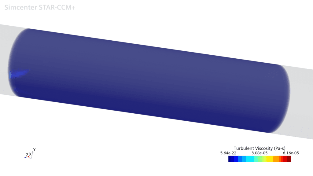
AS for all fields in Simcenter STAR-CCM+, when displaying it, initially there will be a default selection of a colorbar, whatever you have for default, and an adaptation of the scale to capture min and max found on the selected displayed part. Assume we are interested in looking at the turbulent viscosity around and after the sphere in the simulation. The default result for that will look like the picture below shows, completely populating the resampled volume of interest with values. Here we are not really getting any benefits from looking at the 3D-visualization.

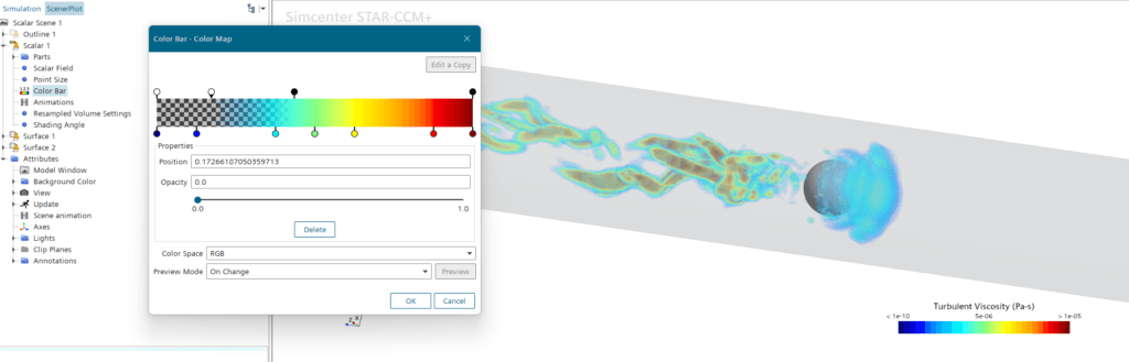
Thera are two major things to consider getting any useful information out of the picture. Those are the range of the scale, and the colorbar. In almost all situations working with the resampled volume, you need limit the scale, and more importantly filter the color bar. Filtering the color bar means simply providing opacity to parts of it. As you can see in the above picture the automatic scale is 17 orders of magnitude different, and that range is often outside of relevance.

In the below picture you can see that by only changing the scale for the colorbar, and by introducing two extra position markers on an editable copy of the used color bar, we can see the turbulent viscosity in a relevant range behind and in front of the sphere. In the edit of the colormap, the two white points show that they have the opacity of 0, meaning that any data between them are not shown. The field between the white and the black marker will have a gradual fade between the opacity values for the two markers respectively.

Manipulating the data for the resampled volume

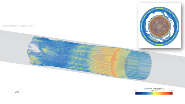
In the case of turbulent viscosity we could use the full resampled volume to show our results on, and the image we see only shows the relevant data in reference to the sphere. But let’s say we are interested in a field that also has values in the relevant range close to the wall. Let’s take turbulent charge for instance. As the picture below shows, even with a manipulated color bar and scale, the result in front of and behind the sphere is blocked by the field values close to the wall. The small picture in the corner shows us that there are data around and behind the sphere that we want to look at. How to deal with this?

The resampled volume can only have a full region as inlet. You cannot use any threshold or a cell set as input for the resampled volume. The issue is that the resampled volume shows little flexibility in its definition and input. And you usually do not want to split our simulation domain into separate regions to make our post processing easier, and nor should you. We don’t do the simulation for the post processing but rather the post processing on the simulation. So, if we cannot impact the resampled volume, we can instead impact the scalar field.

In the method below there is a cylindrical coordinate system created and located in front of the sphere, with the z-axis in the same direction as the global coordinate system and the radial direction following the cylinder radius. By creating a new field function, with the same dimensions as turbulent charge, we can manipulate the scalar field to look like this.

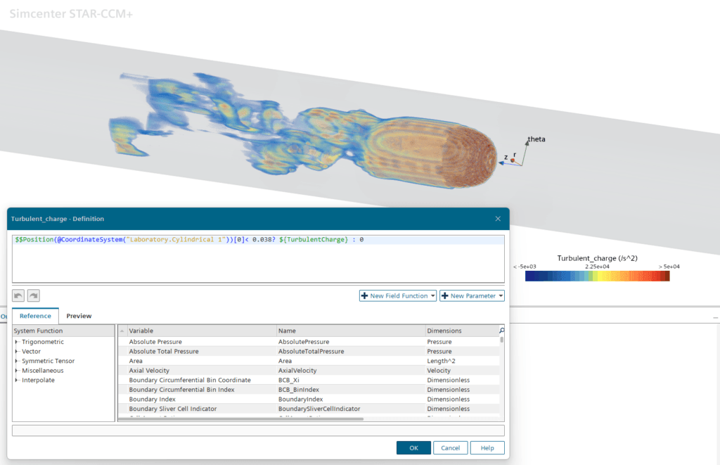
So, while the resampled volume does not have the desired flexibility to isolate results, the scalar field does. By simply creating a scalar field that have the same value as the predefined field of turbulent charge, inside of the radius 3.8 cm and 0 outside, we have isolated the result we are interested in. Alternatively, to achieve the same result you can use a cylindrical shape part with the desired radius and use the function InsidePart(…) to achieve the same thing.

I hope that this has been useful to you, and that you can see the strength of showing results using a resampled volume. As usual, reach out support@volupe.com with any questions.