Courant number (CFL) calculator
Find the Courant number of your time step and cell, or the time step for a target Courant number, checked against the guidance for URANS, LES, free surface and sound.
Courant number and time step calculator
It opens on an LES car wake: 3 mm cells, 30 m/s and a 60 µs step.
Courant number formula
The Courant number, C = |u|Δt/Δx, compares the distance the flow moves in one time step with the size of a cell. |u| is the flow speed through the cell (m/s), Δt the time step (s) and Δx the cell size in the flow direction (m) [1], and C = 1 means that the flow crosses one whole cell per time step.
It is also called the CFL number, after the 1928 paper by Courant, Friedrichs and Lewy that gave the condition behind it [2]. Simcenter STAR-CCM+ reports it as the field function Convective Courant Number [3]. With explicit time stepping it limits stability, and with implicit time stepping it is a guide to accuracy.
How to calculate the Courant number
Take the case the calculator opens with, an LES of a car wake in air at 20 °C. The cells where the eddies are resolved are 3 mm, the local speed is 30 m/s and the time step is 6 × 10⁻⁵ s (60 µs). Equation (1) gives C = 30 × 6 × 10⁻⁵ / 0.003 = 0.60. The flow moves 1.8 mm per step, 0.6 of a cell.
Use the same length unit for the cell and the speed, and C comes out as a pure number. A cell size in millimetres typed as metres makes it a thousand times too small, and the calculator offers the fix when one unit change explains the value.
Time step from a target Courant number
Δt = C Δx / |u| (2)
Turned round, the formula gives the time step for a target Courant number. For the default case and C = 1, Δt = 1 × 0.003 / 30 = 1.0 × 10⁻⁴ s. The same rearrangement gives the smallest cell, |u|Δt/C, or the highest speed, CΔx/Δt, at a given step: 1.8 mm and 50 m/s here.
The flow is often not the only limit, since a shedding period, a rotating part or conduction in a solid can ask for a shorter step, and then the smallest limit sets Δt. The calculator draws each limit as a lane on a time-step budget, and adaptive time-stepping in Simcenter STAR-CCM+ also uses the smallest proposal of its providers [3].
The CFL condition
The CFL (Courant–Friedrichs–Lewy) condition, also called the Courant condition, says that an explicit scheme must not let information travel further in one time step than its stencil reaches, which for first-order upwind means C ≤ 1 [2, 4].
The argument is easiest to follow for a profile φ carried along x at a constant speed u, ∂φ/∂t + u∂φ/∂x = 0, where the exact value at a point comes from a single point a distance ut upstream. An explicit first-order upwind scheme updates each cell from itself and its upstream neighbour, which means that after n steps its answer depends on the n cells upstream [4]. Courant, Friedrichs and Lewy showed that a scheme can only converge if the true domain of dependence lies inside the numerical one [2], which here means uΔt ≤ Δx, or C ≤ 1.
In the figure, after four steps at C = 0.5 the exact value comes from 2 cells upstream, inside the 4 cells the scheme has read. At C = 1.5 it comes from 6 cells upstream, which the scheme never reads, and the shortest wave the mesh can carry, a sawtooth from cell to cell, doubles at every step (our calculation).
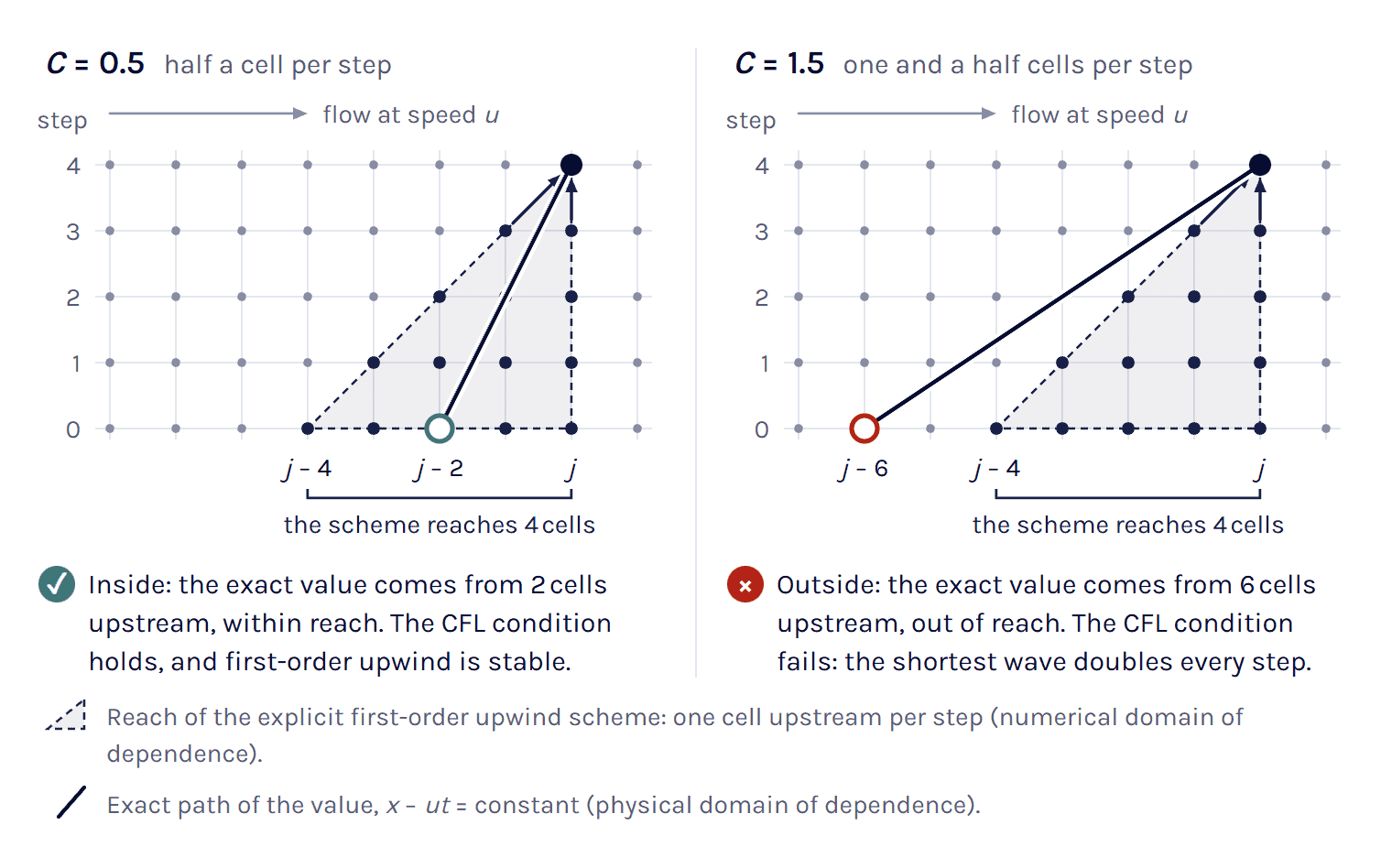
Note that the condition is necessary, not sufficient [4]. Forward Euler with central differences (FTCS) meets it and is still unstable at every Courant number, while first-order upwind is stable for exactly 0 ≤ C ≤ 1 [4].
Explicit stability limits by scheme
C ≤ 1 is the classic limit of the simplest explicit schemes in one dimension, but the limit depends on the scheme and on the number of dimensions. The table comes from a von Neumann analysis as in Trefethen [4]. Rows marked as our calculation apply it to schemes his text does not tabulate.
In two or three dimensions the directions add up, and for first-order upwind the condition becomes
C = Δt (|u|/Δx + |v|/Δy + |w|/Δz) ≤ 1 (3)
(MIT lecture notes give the same sum for 2-D upwind [5], and our von Neumann calculation extends it to 3-D). For flow along a cube diagonal |u|Δt/Δx must then stay below 1/√3 = 0.577. The calculator’s 3-D mode adds up the directions in the same way.
Implicit time stepping and accuracy
Backward Euler and Crank–Nicolson have no Courant limit for linear advection [4], and Jasak notes that Euler implicit stays stable when the explicit limit is broken [6], so with these schemes the time step is chosen for accuracy. When Jasak raised the maximum Courant number of a laminar cylinder run from 0.4 to 2, first-order Euler implicit gave a much lower pressure amplitude and too low a shedding frequency [6].
A DES aeroacoustics tutorial in the Simcenter STAR-CCM+ documentation notes that implicit solvers usually stay stable with local maxima of 10 to 100 if the mean is about 1 [3], but a local value of 50 still means that the flow skips 50 cells per step there. The documentation does warn about PISO: with long time steps it goes unstable once what Siemens calls the combined CFL is well past 10, a point where SIMPLE still runs [3].
Convective vs acoustic Courant number
Equation (1) uses the flow speed, and Simcenter STAR-CCM+ calls it the convective Courant number [3]. In a compressible flow pressure waves also carry information, at the characteristic speeds u, u + c and u − c of the one-dimensional Euler equations, with c the speed of sound [7], and an explicit compressible solver has to meet the CFL condition for the fastest of them
Cac = (|u| + c) Δt / Δx (4)
At the same Courant number and cell, the acoustic step is shorter by the factor (1 + M)/M, with M = |u|/c. In the default case, air at 20 °C with c = 343.3 m/s and M = 0.087, that factor is 12. The acoustic Courant number of the 60 µs step is then 7.5, and an explicit compressible solver would need 8.0 µs. At 10 m/s the factor is 35, and in water at 20 °C (c = 1483 m/s) at 2 m/s it is 743 (our arithmetic).
The explicit solver in Simcenter STAR-CCM+ works on this number. Explicit Unsteady needs the coupled solver with the Coupled Energy model and inviscid or laminar flow, and it picks one time step for the whole domain that keeps the Courant number on flow speed plus speed of sound at 1 or below [3]. The documentation writes the explicit step as the cell volume over the largest eigenvalue (flow speed plus speed of sound, times a face area) but does not say how the faces of a cell add up in it [3], so in its 3-D mode the calculator sums (|ui| + c)Δt/Δxi over the three directions, as the local time-step routine of the open-source solver ADflow does [8]. That sum is our estimate of the explicit limit.
Which cell size and which velocity
Δx is the cell length in the direction the flow goes through it, the linear cell size in the flow direction in the ITTC guideline [1], which on a hexahedral cell lined up with the flow is the edge along the flow. A polyhedral cell has no such edge, and for a compact one we use the cube root of the volume as our hand estimate.
In prism layers the choice of length matters most, because a wall cell can be a hundred times longer along the wall than it is thick. Take a cell 2 × 2 mm along the wall and 0.02 mm thick, with 5 m/s parallel to the wall and Δt = 0.1 ms. On the length along the flow C = 0.25, on the cube root of the volume 1.16 and on the thickness 25 (our calculation), so for flow along a wall use the length along the wall and keep the thickness for the diffusion number.
Codes do not all report the same number for the same cell. OpenFOAM, for example, uses half the sum of the volume fluxes through the faces, times the time step, over the cell volume [16], which for flow along a cube diagonal gives √3 = 1.73 times |u|Δt/Δx. The original HRIC paper uses one face over the donor-cell volume [17], 0.58 on the same cell (our calculation), and Simcenter STAR-CCM+ does not give the discrete formula of its field function [3]. Compare a value with a guideline only when both use the same definition.
For |u|, take the speed in the cells you check, not the inlet speed. In the focus region of a DES grid Spalart takes the highest speed as typically 1.5 to several times the free-stream speed [18]. On a moving mesh use the velocity relative to the mesh, as Simcenter STAR-CCM+ does [3]. Near a fan tip in still air that is about the tip speed 2πrn.
Guides also take the number in different places: Siemens an average over the zone of interest [3], ITTC the local value [1] and OpenFOAM’s adjustable time step the largest value in the mesh [16], and a run can meet one of them and miss another.
Courant number targets by case
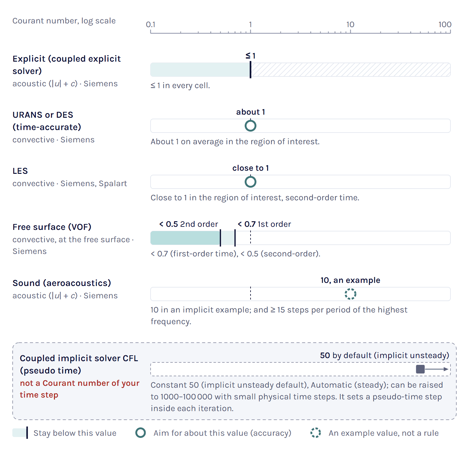
Explicit solvers have a stability limit, and implicit solvers a guide to accuracy that depends on what you resolve. The table gives each target with its owner and the number it refers to.
URANS and DES
Siemens’ guidance for time-accurate runs is a convective Courant number of about 1 on average in the zone of interest, where the flow moves about one cell per step, and the documentation presents it as an indication for choosing the step rather than a hard limit [3]. For vortex shedding the documentation also points to the Strouhal number [3], so count the steps per period as well and take the smaller step.
LES
For LES, Siemens asks for a convective Courant number close to 1 in the domain of interest, with second-order time [3]. Spalart reaches the same local value from accuracy for the focus region of a DES grid, where the smallest active eddies span about five cells and a scheme of at least second order needs about five steps per period, so Δt = Δ0/Umax [18]. He adds that steps 1.5 or even 2 times longer or shorter cannot be called incorrect.
Free surface (VOF)
The VOF guidelines in Simcenter STAR-CCM+ ask for a Courant number below 0.7 with first-order time and below 0.5 with second-order time, at any cell face in the free-surface zone [3]. With second-order time a surface that moves half a cell or more per step can overshoot, and the run can diverge [3]. HRIC also blends towards first-order upwind between CFL_l = 0.5 and CFL_u = 1 by default, which smears the interface [3] (the original paper used 0.3 and 0.7 [17]). For a steady answer both are set high, for example 50 and 100 [3], as our post Insights in VOF interface capturing: HRIC vs MHRIC shows on a ship hull.
Sound
Siemens’ aeroacoustics guidelines take the smallest of several limits: at least 15 steps per period of the highest frequency of interest F, Δt ≤ 1/(15F), and an acoustic CFL on the flow speed plus the speed of sound, which an implicit example in the guidelines sets to 10 [3].
Steady runs and the coupled solver’s CFL
A steady run has no physical time step, and the convective Courant number therefore does not apply [3]. The coupled solver’s CFL setting, Automatic in steady runs and a constant 50 in implicit unsteady runs by default, sets a pseudo time step inside the solver and is not the Courant number of your time step [3]. Our posts Solving the engineering question and Coupled solver settings in Simcenter STAR-CCM+ explain the difference.
Check the step by halving it
Whatever the target, check that the answer you need does not change when you halve the time step, as our dimensionless numbers page also says. In the valve case of our post Solving the engineering question the opening time was 5.1 ± 0.1 ms for steps of 10⁻⁴, 10⁻⁵ and 10⁻⁶ s, so the longest step was enough for that question. In a transient case, find the step this way on one mesh first and then run the grid study in the GCI calculator with that step fixed, as its page describes.
Periodic flow and rotating parts
A periodic flow also needs enough steps per period, and with f the frequency that number is
N = 1 / (f Δt) (5)
Siemens’ segregated-flow guidelines suggest about 50 to 100 steps per period, and for the coupled implicit solver the documentation sets more than two steps, the Nyquist criterion, as the floor [3]. ITTC asks for at least 100 for periodic phenomena such as vortex shedding, and at least 20 per period of the highest frequency in complex unsteady flows [1].
The time scheme also decides how much of the amplitude survives. For a pure oscillation with no error in space, backward Euler keeps 39 % of the amplitude per period at 20 steps, 61 % at 40 and 82 % at 100, where BDF2 keeps 96 %, 99.4 % and 99.96 % (our calculation).
For rotating parts count the degrees per step, 360nΔt with n in revolutions per second. The Simcenter STAR-CCM+ documentation suggests about 1° per step for rotating blades in several places, among them the blade element method, a rotating-fan tutorial and axial-fan acoustics [3]. ITTC asks for at least 180 steps per propeller revolution, 2° per step, where its 2011 version asked for 200 [1, 19].
Axial-fan acoustics also asks for at least 15 steps per blade passage, which is tighter than 1° per step above 24 blades [3]. On an overset mesh, keep the motion per step in the overlap below the smallest cell there with first-order time, and below half of it with second-order time [3].
Diffusion number and conjugate heat transfer
Diffusion has a number of the same kind, built from the diffusivity D, which is ν for momentum and α = k/(ρcp) for heat
d = D Δt / Δx² (6)
For heat it is the cell Fourier number, Fo in our post on time-step selection in conjugate heat transfer, and Simcenter STAR-CCM+ calls it the von Neumann number of thermal diffusivity [3]. Note that Δx is squared, which means that halving the cell quarters the step for the same d, where the Courant number only halves it.
For the heat equation the explicit stability limit is d ≤ 1/2 in 1-D with forward Euler and central differences [4], and with equal spacing in n dimensions it is 1/(2n) (our von Neumann calculation, the same limits as in our CHT post). Engineers often call this the CFL condition for the heat equation, although it comes from a von Neumann analysis rather than from the domain of dependence [4]. Implicit solvers have no such limit, and for them the Thermal Diffusivity provider in Simcenter STAR-CCM+ aims at 0.5 on average and 5 at most by default [3], while our CHT post takes about 1 or less as a rule of thumb.
In that post an aluminium block cooled by a flow of 0.02 m/s gets almost the same step from both numbers with 5 mm cells, 0.25 s and 0.26 s. The post takes Δt = min(Δtflow, Δtdiff), as adaptive time-stepping does with its providers [3], and with 2.5 mm cells the solid wins (the CHT example below).
The viscous diffusion number can matter as well, mainly in thin wall cells. Cells 10 µm thick in water at 20 °C with Δt = 0.1 ms give a viscous d of 1.0, twice the explicit 1-D limit (our calculation), and the ratio C/d = |u|Δx/D, the cell Péclet number, tells you which of the two limits is closer.
Worked examples
LES of a car wake
The default case gives C = 0.60, a little below Siemens’ LES guidance of close to 1 [3] and within the factor of 2 that Spalart says cannot be called incorrect [18]. Halve the wake cells to 1.5 mm and the same 60 µs step gives C = 1.2, so a finer mesh needs a shorter step, here 50 µs for C = 1.
Load the LES example in the calculator ↑
Vortex shedding: convection or period?
Take a 20 mm cylinder in air at 5 m/s (Re = 6640), run as URANS with 0.5 mm cells in the wake and the free-stream speed taken as the typical speed there. Roshko found St essentially constant at about 0.21 up to Re = 10⁴ [20], which gives f = St·U/D = 0.21 × 5 / 0.02 = 52.5 Hz. Fifty steps per period, the low end of Siemens’ range, allow 3.8 × 10⁻⁴ s [3]. A Courant number of 1 in the wake needs 1.0 × 10⁻⁴ s, about 190 steps per period, and convection therefore sets the step, as in Siemens’ DES cylinder tutorial [3].
Load the vortex-shedding example in the calculator ↑
Free surface with second-order time
Consider water at 20 °C with 5 mm cells at the interface, a surface speed of 2 m/s and second-order time. The target of 0.5 gives Δt = 0.5 × 0.005 / 2 = 1.25 × 10⁻³ s, and first-order time with 0.7 would allow 1.75 × 10⁻³ s [3]. Implicit multi-stepping divides the global Courant number at the interface by the number of sub-steps. With second-order time, multi-stepping updates only the convective term in the sub-steps, and the Segregated VOF Solver reference notes that the global Courant number can then typically be 2 to 3 times higher while the local value stays at about 0.1 to 0.3 [3]. Doubling the step to 2.5 × 10⁻³ s, a global C of 1.0, therefore takes 4 sub-steps of C = 0.25, if the rest of the physics allows the longer step. The solver’s own dynamic mode defaults to a target sub-step CFL of 0.5 and at most 20 sub-steps [3].
Load the free-surface example in the calculator ↑
Explicit run at high speed
Here an explicit solver runs air at 20 °C at 250 m/s, with 1 mm as the smallest cell. The flow speed alone would allow 4.0 µs, but Cac = 1 allows only 1.69 µs at M = 0.73, and at that step the convective C is only 0.42.
Load the high-speed example in the calculator ↑
Fan at 2000 rpm
The fan has a tip radius of 250 mm, runs at 2000 rpm and has 9 blades and 5 mm cells at the tip. One degree per step gives Δt = 1/(6 × 2000) = 8.33 × 10⁻⁵ s, the value in the rotating-fan tutorial of the Simcenter STAR-CCM+ documentation [3]. That is 360 steps per revolution and 40 per blade passage. At the tip speed of 52.4 m/s the step gives C = 0.87. An overset rotor would move 0.87 of a tip cell per step, inside the first-order rule but not the second-order one [3].
Load the fan example in the calculator ↑
CHT block from our blog
This is the aluminium block from our post on time-step selection in conjugate heat transfer, now with 2.5 mm cells and the same flow of 0.02 m/s. The flow allows 0.125 s at C = 1 and the solid 0.064 s at Fo = 1, so conduction sets the step. The Thermal Diffusivity provider’s default mean target of 0.5 [3] halves it to 0.032 s.
Courant number in Simcenter STAR-CCM+
In Simcenter STAR-CCM+ the Courant number of your time step is the field function Convective Courant Number, with the velocity relative to the mesh when the mesh moves, and it only means something in unsteady runs [3]. Our post Solving the engineering question explains how it differs from the coupled solver’s CFL. Show the Convective Courant Number in a scalar scene and add a Maximum report on it as a monitor and plot [3], and note that the built-in report called Courant Number returns the coupled solver’s CFL instead [3].
The Implicit Unsteady solver starts at 0.001 s and first-order time unless you change them [3]. In the optional Adaptive Time-Step model the CFL provider aims at a Target Mean CFL Number of 0.5 and a Target Max CFL Number of 5.0 by default, and the Thermal Diffusivity and Free Surface CFL providers do the same job for conduction and free surfaces [3].
The calculator’s panel lists these settings for your case. For help with a set-up, use the form below and choose Technical question.
References and changelog
References
[1] ITTC Recommended Procedures and Guidelines 7.5-03-02-03, Practical guidelines for ship CFD applications, Revision 01, effective 2014, section 3.6 Time step. https://www.ittc.info/media/8165/75-03-02-03.pdf
[2] R. Courant, K. Friedrichs and H. Lewy, Über die partiellen Differenzengleichungen der mathematischen Physik, Mathematische Annalen 100, 32–74, 1928. English translation: On the partial difference equations of mathematical physics, IBM Journal of Research and Development 11(2), 215–234, 1967. https://doi.org/10.1147/rd.112.0215
[3] Simcenter STAR-CCM+ documentation, version 2606, Siemens Digital Industries Software, 2026: Field Function Library, System Reports, Time and Adaptive Time-Stepping, Segregated and Coupled Flow Solver guidelines, the Volume of Fluid theory (HRIC), VOF Guidelines, Multi-Stepping Guidelines and the Segregated VOF Solver reference, LES Guidelines, Overset Mesh Workflow, Virtual Disk (Blade Element Method), Guidelines for Aeroacoustics Calculations, and the tutorials Rotating Fan and DES and FW-H On-The-Fly: Noise from a Cylinder.
[4] L. N. Trefethen, Finite Difference and Spectral Methods for Ordinary and Partial Differential Equations, unpublished text, Cornell University, 1996, sections 1.9 and 4.3–4.4. https://people.maths.ox.ac.uk/trefethen/pdetext.html
[5] MIT OpenCourseWare, 12.950 Atmospheric and Oceanic Modeling, Spring 2004, lecture notes 10, Advection in two dimensions, sections 6.1–6.2. https://ocw.mit.edu/courses/12-950-atmospheric-and-oceanic-modeling-spring-2004/
[6] H. Jasak, Error Analysis and Estimation for the Finite Volume Method with Applications to Fluid Flows, PhD thesis, Imperial College London, 1996, sections 3.3 and 6.5.
[7] J. L. Steger and R. F. Warming, Flux vector splitting of the inviscid gasdynamic equations with application to finite difference methods, NASA TM-78605, 1979 (Journal of Computational Physics 40, 263–293, 1981). https://ntrs.nasa.gov/citations/19790020779
[8] MDO Lab, University of Michigan, ADflow source code, src/solver/solverUtils.F90, subroutine timestep_block, read October 2026. https://mdolab-adflow.readthedocs-hosted.com/en/stable/_static/doxydoc/html/dc/d8c/solver_utils_8_f90_source.html
[9] E. W. Lemmon, R. T Jacobsen, S. G. Penoncello and D. G. Friend, Thermodynamic properties of air and mixtures of nitrogen, argon, and oxygen from 60 to 2000 K at pressures to 2000 MPa, Journal of Physical and Chemical Reference Data 29(3), 331–385, 2000. https://doi.org/10.1063/1.1285884
[10] IAPWS R7-97(2012), Revised Release on the IAPWS Industrial Formulation 1997 for the Thermodynamic Properties of Water and Steam.
[11] IAPWS R6-95(2018), Revised Release on the IAPWS Formulation 1995 for the Thermodynamic Properties of Ordinary Water Substance for General and Scientific Use.
[12] ITTC Recommended Procedures and Guidelines 7.5-02-01-03, Fresh water and seawater properties, International Towing Tank Conference, 2011.
[13] N. P. Fofonoff and R. C. Millard, Algorithms for computation of fundamental properties of seawater, Unesco Technical Papers in Marine Science 44, 1983, section 9 (speed of sound after C.-T. Chen and F. J. Millero, 1977). https://doi.org/10.25607/OBP-1450
[14] E. W. Lemmon and R. T Jacobsen, Viscosity and thermal conductivity equations for nitrogen, oxygen, argon, and air, International Journal of Thermophysics 25(1), 21–69, 2004.
[15] IAPWS R15-11, Release on the IAPWS Formulation 2011 for the Thermal Conductivity of Ordinary Water Substance, 2011.
[16] OpenFOAM Foundation, OpenFOAM-dev source code (CourantNo.H, setDeltaT.H) and the damBreakLaminar tutorial, read October 2026. https://github.com/OpenFOAM/OpenFOAM-dev
[17] S. Muzaferija, M. Perić, P. Sames and T. Schellin, A two-fluid Navier–Stokes solver to simulate water entry, Proceedings of the 22nd Symposium on Naval Hydrodynamics, Washington, D.C., 1998, National Academy Press, 1999, 638–651. https://doi.org/10.17226/9771
[18] P. R. Spalart, Young-person’s guide to detached-eddy simulation grids, NASA/CR-2001-211032, 2001, section 2.6. https://ntrs.nasa.gov/citations/20010080473
[19] ITTC Recommended Procedures and Guidelines 7.5-03-02-03, Practical guidelines for ship CFD applications, effective 2011, section 2.5 Choice of the time step. https://www.ittc.info/media/1357/75-03-02-03.pdf
[20] A. Roshko, On the development of turbulent wakes from vortex streets, NACA Report 1191, 1954. https://ntrs.nasa.gov/citations/19930092207
Changelog
October 2026: first published, with the calculator and this guide. The targets, stability limits and fluid properties were checked against the sources listed above.
Questions about the Courant number
Ask a Volupe specialist
Christoffer Johansson
Senior Application Specialist, M.Sc.
Questions about time steps, Courant numbers or solver settings? We reply within one day.
Ask a technical question →
What is the Courant number in CFD?
The Courant number C = |u|Δt/Δx compares how far the flow moves in one time step with the size of a cell. C = 1 means that the flow crosses one whole cell per step. It is also called the CFL number, after the 1928 paper by Courant, Friedrichs and Lewy. With explicit time stepping it is a stability limit, and with implicit time stepping a guide to accuracy.
What is the formula of CFL?
C = |u|Δt/Δx, with |u| the flow speed through the cell in m/s, Δt the time step in s and Δx the cell size in the flow direction in m. Turned round, Δt = CΔx/|u| gives the time step for a target C. An explicit compressible solver uses the acoustic Courant number (|u| + c)Δt/Δx, with c the speed of sound. In three dimensions first-order upwind needs the sum over the directions, Δt(|u|/Δx + |v|/Δy + |w|/Δz), to stay at or below 1.
How do you calculate the Courant number?
Multiply the speed by the time step and divide by the cell size, all in SI units. At 30 m/s, a time step of 6 × 10⁻⁵ s and 3 mm cells, C = 30 × 6 × 10⁻⁵ / 0.003 = 0.6, so the flow moves 0.6 of a cell per step. Use the speed in the cells you care about rather than the inlet speed, and on a moving mesh the speed relative to the mesh.
What is a good CFL number?
With an implicit solver, Siemens suggests a Courant number of about 1 on average in the zone of interest for time-accurate runs, close to 1 for LES, and below 0.7 with first-order time or 0.5 with second-order time at a VOF free surface. With an explicit solver C has to stay within the stability limit of the scheme, 1 for the simplest schemes and for the explicit solver in Simcenter STAR-CCM+, where it includes the speed of sound. Whatever you pick, check that the answer you need does not change when you halve the time step.
What does CFL mean in CFD?
CFL stands for Courant–Friedrichs–Lewy, after the authors of a 1928 paper on difference equations. The CFL condition, also called the Courant condition, says that an explicit scheme can only converge if its numerical domain of dependence contains the true one, so in one time step the flow must not move further than the stencil reaches. For first-order upwind that means C ≤ 1. The condition is necessary but not sufficient for stability.
Can the Courant number be greater than 1?
Yes. With an implicit solver backward Euler has no Courant limit for linear advection, and a DES tutorial in the Simcenter STAR-CCM+ documentation notes that implicit solvers usually stay stable with local maxima of 10 to 100 if the mean is about 1. Accuracy suffers, though, and with long time steps PISO goes unstable once what Siemens calls the combined CFL is well past 10, while SIMPLE still runs. A second-order free-surface run can also diverge once the surface moves half a cell or more per step. Some explicit schemes also allow more than 1, such as four-stage Runge–Kutta with central differences (2.83 in the linear model), but above the limit of its scheme an explicit run is unstable.
How do I choose the time step from the Courant number?
Rearrange the formula: Δt = CΔx/|u| for your target C. With 3 mm cells, 30 m/s and a target of 1, Δt = 0.003/30 = 1 × 10⁻⁴ s. Then check the other limits of the case, such as the steps per period of a shedding wake, the degrees per step of a rotating part or the diffusion number of a solid, and take the smallest step.
Is the CFL number in Simcenter STAR-CCM+ the same as the Courant number?
Not always. The field function Convective Courant Number is the Courant number of your time step. The CFL setting of the coupled solver, a constant 50 by default in implicit unsteady runs and Automatic in steady runs, sets a pseudo time step inside the solver, and the built-in report called Courant Number shows that setting. The Target Mean and Target Max CFL Numbers of the adaptive time-step CFL provider, 0.5 and 5.0 by default, do refer to the convective Courant number.
Can Volupe help me set up time steps in Simcenter STAR-CCM+?
Yes. Our application engineers help Simcenter STAR-CCM+ users with set-ups like these, from the time model and the time step to adaptive time-stepping and the mesh. Customers with maintenance get this through our support, and we also run Simcenter STAR-CCM+ training courses.