Pump curve and NPSH calculator
Find where your pump runs on your system, its NPSH margin and the speed a new flow needs.
Calculator
Pump curve and system curve: finding the operating point
The operating point (often called the duty point) is the flow and head at which the pump curve crosses the system curve: there the pump gives exactly the head the system needs [1, 2]. The calculator finds it from three relations, which are also what you would use by hand.
Hpump(Q) = Hsys(Q) = Hst + hs(Q) + hd(Q) (1)
NPSHa = (ps − pv)/(ρg) + zs − hs(Q) (2)
Q2/Q1 = n2/n1, H2/H1 = (n2/n1)2, P2/P1 = (n2/n1)3 (3)
In (1) Hst is the static head and hs and hd are the losses in the suction and discharge lines. In (2) ps is the absolute pressure on the suction surface, pv the vapour pressure of the liquid and zs the height of the suction surface above the impeller centre, negative when the pump sits above it [3]. (3) are the affinity laws for a change of speed from n1 to n2 [4].
A pump curve, also called the performance curve or characteristic, gives the head H a pump adds to the liquid against the flow Q for one speed of the pump [5]. In the calculator it is the table from the data sheet: 3 to 8 points of flow and head, with NPSH3 and efficiency where you have them. The curve drawn through them passes through every point you type and cannot add a hump that the points do not show [6]. With three points the shape between them is a guess, so type five or more where the data sheet gives them. The test curves behind that advice are under How the calculator works. Beyond the first and the last point the curve is extended by a straight line for at most 10 % of the last flow, never below zero flow, and a point found on an extension is flagged.
The system curve is the head the piping needs at each flow: the static head plus the friction and fitting losses of the suction and discharge lines [7]. The static head is its value at zero flow, the difference in level between the two liquid surfaces plus their pressure difference as a head [7]. At your flow, the system curve gives the head the pump has to deliver, commonly called the total dynamic head (TDH). Maurer finds the total dynamic head from the energy equation between the two liquid surfaces, with the velocity at both surfaces negligible [8]. We do the same: the static head holds the two levels and the two tank pressures, and no velocity head at the surfaces. For each line the calculator works out the friction factor again at every flow, with the same code as our Moody chart and pipe pressure drop calculator, and adds the loss coefficients ΣK, which you can sum from the table of K values there. Because the surfaces carry no velocity head, ΣK has to hold the entrance from the suction tank and the exit into the discharge tank as well as the fittings. The default lines hold both, with the values from that table: K = 0.8 for a suction pipe end that projects into the tank, and K = 1 at the exit into the discharge tank, where the whole velocity head is lost.
For water in steel pipe, working out f again at every flow changes little compared with the textbook shortcut, a parabola kQ2 on top of the static head [2]. In the default case the parabola through the operating point lies 0.16 m below the recalculated curve at 21 m³/h and 0.45 m above it at 60 m³/h (our calculation). The difference grows where the friction factor changes faster with flow, as it does for viscous liquids in laminar flow (our reasoning). If you only know one duty point, the One duty point mode draws that parabola through it.
How to read a pump curve
Start from the flow you need on the flow axis, which the head, efficiency, power and NPSH curves share. Go up to the head curve and read the head at your flow, at the one speed it holds for [5]. Read the efficiency there and see how far you are from the best efficiency point (BEP), the top of the efficiency curve [9]. Read the power the same way: it usually rises with flow on a radial pump and falls on an axial one [9]. Last, read NPSH3 (NPSHr) at your flow. The maker lowers the suction head at constant flow until the head drops by 3 %, and repeats this at several flows [2].
At a lower speed the head and power curves move down and to the left, and the efficiency curve moves left [9]. A maker usually gives a pump a curve for each impeller size it offers, and a coverage chart describes a whole family of pumps [9]. This pump curve calculator needs only one of these curves: head against flow at the data-sheet speed, with NPSH3 and efficiency where you have them. It works out power from head and efficiency [10] and scales the curve to another speed or a trimmed impeller.
The default case worked through
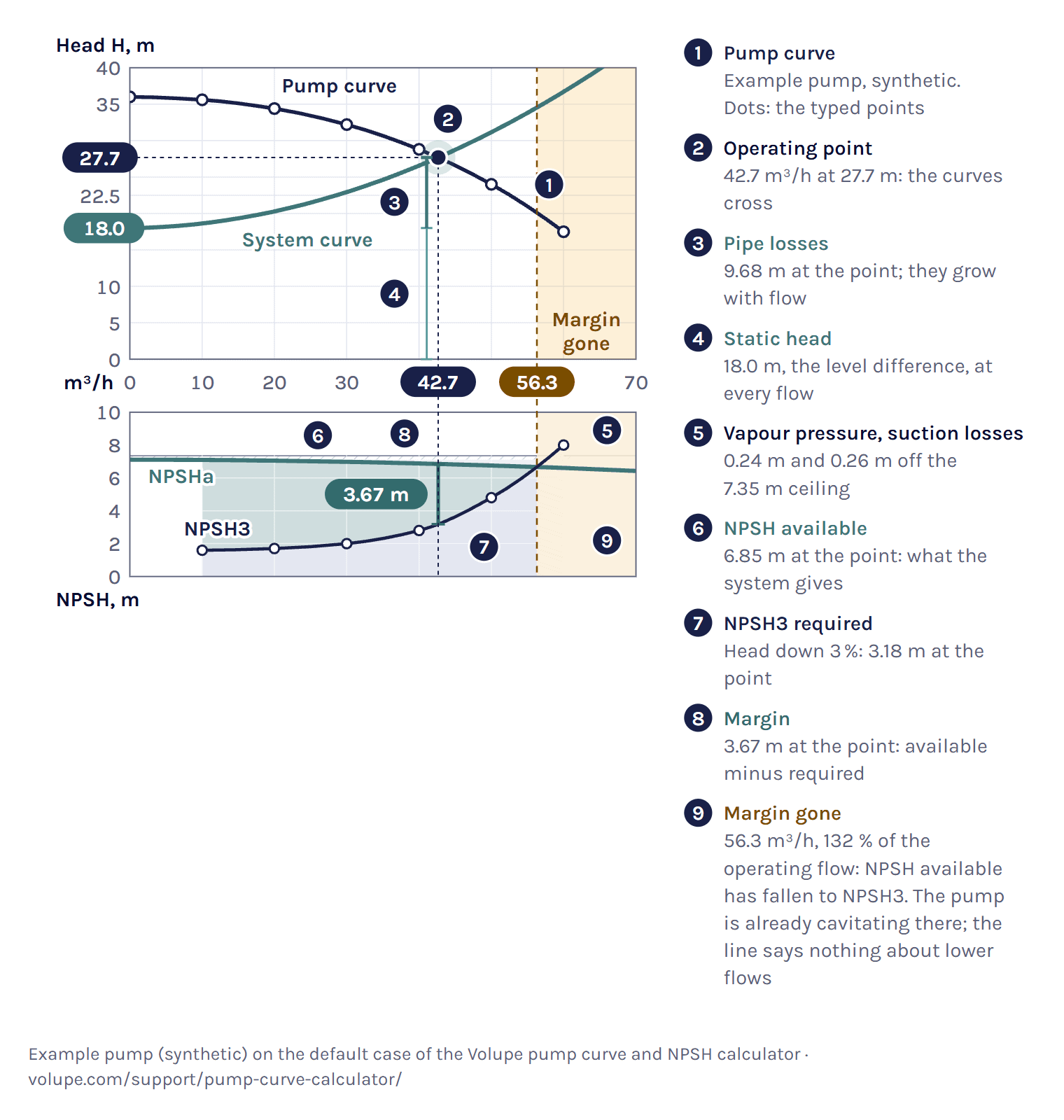
Unless it is marked otherwise, every number for the example pump on this page is the calculator’s own result, as you get it when you load the example. The calculator opens on a synthetic pump, not a maker’s: seven points from 36.0 m at no flow down to 17.5 m at 60 m³/h. It pumps water at 20 °C between two open tanks at sea level, with the discharge level 18.00 m above the suction level and the pump 3 m above the suction level. The suction line is 6 m of 100 mm steel pipe with ΣK = 1.1, the discharge line 120 m of 80 mm steel pipe with ΣK = 4.4, both with a roughness of 0.045 mm.
The curves cross at 42.7 m³/h and 27.7 m. Of the 27.68 m, 18.00 m is static, 9.42 m is lost in the discharge line and 0.26 m in the suction line. The typed efficiency points give 77 % there, so the pump gives the water ρgQH = 3.21 kW of hydraulic power [4] and takes 4.18 kW at the shaft, the hydraulic power divided by the efficiency [10]. Under the result you also see the operating flow as a share of the flow at the best typed efficiency, here 107 %. We show it as a number only, because whether that is far enough from the best point depends on the pump.
A curve whose head first rises from shut-off and then falls, a drooping curve, is unstable in the rising part [11], and against a high static head it can cross the system curve twice. In the drooping example the static head is 30.50 m against a shut-off head of 30.0 m, and the curves cross at 3.00 m³/h and 15.1 m³/h. The calculator takes 15.1 m³/h, where the pump curve crosses the system curve from above, and warns that the pump cannot start the flow against this static head on its own. We show why the crossing from above is the stable one in our derivations at the end of How the calculator works.
Load the drooping-curve example in the calculator ↑
How to draw a pump curve
Take the head and flow pairs from the data sheet at the speed the sheet is for, and the NPSH3 and efficiency values at the same flows if they are given. Paste them with Paste from a data sheet or type them into the table, 3 to 8 rows. The calculator draws the curve through every point, puts NPSH3 on the panel below on the same flow axis and marks the best efficiency of the typed points. Then add the system: the two levels and the two pipe lines, or one duty point. Download chart gives the chart with your case as an SVG file. It also gives the blank pump curve sheet as an A4 image for print.
To draw one by hand, use the blank sheet below: plot the points, then draw one smooth line through them that only turns where a point turns, and stop at the last point, because past it you have no data. The calculator goes at most 10 % further and flags a point found there. The NPSH grid under the head grid shares its flow axis, so NPSH3 reads at the same flow as the head.
NPSH available and NPSH required
For NPSH available you need no pump curve, only the suction side, so the calculator also works as a plain NPSH calculator. Under Find, choose NPSH margin at a flow you give, then type the flow and the suction side. On the default suction side at 40.0 m³/h NPSH available is 6.88 m. Add the NPSH3 the data sheet gives at that flow, 2.80 m for the default pump, and you also get the margin, 4.08 m, and the ratio, 2.46.
NPSH available (NPSHa) is the total head at the pump inlet above the vapour-pressure head of the liquid, referred to the impeller centre [3]. NPSH required (NPSHr), given on data sheets as NPSH3, is the NPSH at which the pump’s head has dropped by 3 % because of cavitation [3]. It is NPSH3 by common agreement because showing where cavitation begins takes demanding and expensive testing [3]. NPSH available belongs to your suction side, and we work it out from (2). NPSH3 belongs to the pump, so you type it from the data sheet.
Read (2) as a budget from the suction surface to the pump inlet: what the atmosphere gives, minus what the height, the suction line and the vapour pressure take [3]. In the default case the atmosphere at sea level holds up 10.35 m of water at 20 °C. The pump sits 3 m above the surface, which takes off 3.00 m. The suction line loses 0.26 m at the operating flow and the vapour pressure takes 0.24 m. That leaves NPSH available of 6.85 m, against the 3.18 m the pump needs at that flow. The margin of 3.67 m runs out at 56.3 m³/h, 132 % of the operating flow, because the example’s NPSH3 column rises steeply above 40 m³/h while NPSH available falls only slowly with flow.
The velocity head at the inlet, 0.12 m here, is already part of NPSH available [3]. The energy balance from the surface accounts for it, so it is not taken off again.
At altitude the atmosphere holds up less. We take the pressure on an open tank from the U.S. Standard Atmosphere 1976 for the altitude you give [12]: 79.5 kPa at 2000 m instead of 101 325 Pa at sea level, which agrees with KSB’s table to three figures [13]. With both tanks at 2000 m the default pump has 4.62 m of NPSH available instead of 6.85 m. The real pressure varies with place and weather, and KSB uses the averaged value for rough calculations only [13], so if you know it, type it as the tank pressure. The same altitude sets the atmosphere for a gauge reading on a closed tank. One standard atmosphere at 2000 m would overstate NPSH available by 2.23 m (our calculation).
For water the calculator takes the vapour pressure, the density and the viscosity at the temperature you give from IAPWS-IF97 and the IAPWS 2008 viscosity formulation, 0 to 350 °C [14, 15]. At 20 °C that is 2.34 kPa, 998.2 kg/m³ and 1.002 mPa·s. Our air and water properties calculator gives the density and viscosity of water with the same formulations, and the temperature at which it boils at a given pressure.
A closed tank holding liquid at its boiling point has ps = pv, so (2) leaves only the height of the level above the pump minus the suction losses. In the closed-tank example, saturated water at 105 °C with the pump 6 m below the level, that is 5.72 m against 3.77 m required, a margin of 1.95 m.
KSB puts the theoretical limit of suction lift for water at 10.33 m, under ideal conditions. In practice the lift is less, because the suction-line friction and the vapour pressure take their share [16], and so does the pump’s own NPSH required, as (2) shows when you set NPSH available equal to it. How much is left depends on your suction line, your liquid and your pump, so the Suction limit mode under Find works it out for your own case.
Pump cavitation and the NPSH margin
Cavitation is the formation and collapse of vapour bubbles on the impeller, as the local pressure falls below the vapour pressure of the liquid and rises above it again [5]. Most centrifugal pumps cannot stand it for long: the impeller erodes or the pump vibrates, although some pumps are designed to run with limited cavitation [5].
The NPSH margin is NPSH available minus NPSH required at the operating flow, and the NPSH ratio is the one divided by the other. The calculator gives both, 3.67 m and 2.15 in the default case, and marks the point where NPSH available falls to NPSH3, the 3 % head drop.
Note that a margin of zero does not mean the pump is free of cavitation. At that point the pump is already cavitating and its head is down by 3 % [17], because cavitation begins at a higher NPSH, the incipient value NPSHi [3]. 3 % was chosen because it was the smallest head drop that could be measured consistently [17]. The point says nothing about lower flows: a pump can also cavitate at part load while NPSH available is still above NPSH3, because NPSHi has its lowest value near the shock-free flow and rises again towards low flow [3]. We do not estimate where cavitation begins: as KSB says, that takes testing [3]. Below NPSH required, cavitation lowers the flow and the head, and flow and discharge pressure fluctuate [2].
We do not lower the pump curve for this. Wherever NPSH available is at or below NPSH3, the calculator tints the chart and keeps the curve as you typed it. The band where the margin runs out carries the label Margin gone. In the default case it starts at 56.3 m³/h, 132 % of the operating flow, and it is the only one. If the operating point falls in a tinted band, its head comes from the typed curve, and the pump will not reach it there.
A higher temperature raises the vapour pressure and takes the margin away. In the hot-water example, at 85 °C with the pump 3 m above the level, NPSH available is 1.32 m against 3.30 m required, a margin of −1.98 m. The Suction limit mode gives the way back: at 85 °C the pump may sit at most 1.02 m above the level, or with the pump at 3 m the water may be at most 75.1 °C. Keeping 0.5 m, the low end of Grundfos’s allowance [2], brings that down to 71.9 °C.
Load the hot-water example in the calculator ↑
What margin to keep
We do not judge your margin, because no single value fits every pump. The table lists what named sources recommend. The Hydraulic Institute adds that a pump needs more margin when it runs outside its preferred operating region around the best efficiency point [17].
Type a target under Margin to keep, in metres or as a ratio, and the status shows whether you keep it. Without a target we show the numbers and no verdict. With the 25 % rule the default pump could sit up to 5.87 m above the suction level. Grundfos looks past the operating point: it reads NPSH required at the highest flow the pump will run at when it works out the suction lift [2]. The sourcebook asks for its 25 % at all expected flows [9]. So type your highest expected flow under NPSH margin and read the margin there too.
Affinity laws: speed and impeller diameter
The affinity laws scale a pump curve with speed: flow with the speed ratio, head with its square and power with its cube, as in (3) [4]. They hold strictly for frictionless, incompressible flow without cavitation [4], and the power law assumes the efficiency does not change. Fans follow the same laws: flow with speed, pressure with its square and power with its cube [21].
The laws move every point of the pump curve, not the operating point. The new operating point is where the scaled pump curve meets the system curve, and it follows the laws only when the system curve is a parabola through the origin, with no static head [2]. With static head, a lower speed moves the pump towards shut-off [9].
The default system has 18.00 m of static head in its 27.7 m. To get half the flow, 21 m³/h, the affinity laws alone say 49.2 % speed. At that speed the pump’s shut-off head is 8.73 m, below the static head, so the pump moves no water at all. Against the real system curve the Speed mode under Find gives 78.8 %. Below 70.7 % this pump moves nothing against 18.00 m, because its shut-off head of 36.0 m times the speed ratio squared falls below the static head (our derivation).
At reduced speed we keep the efficiency of the matching point on the full-speed curve, which is an approximation. Grundfos gives its efficiency estimate as valid down to 50 % speed [2], and below that the calculator warns. It does not run the pump above 100 % of the data-sheet speed.
NPSH required is scaled with speed by default as head is: read at Q/r and multiplied by r2, where r is the speed ratio. This is the least certain part of a speed change. A TU Delft test series on a dredge pump found the square law, and notes that Gülich and Yedidiah use an exponent below 2 [22]. A pump consultant gives 1.7 to 2.0 [23], and KSB lists converting NPSH to another speed among the cases that need a test [3]. With an exponent below 2 the square law gives the lower NPSH required at reduced speed, so the margin shown there is the optimistic end. At 80 % speed and 32 m³/h the default pump needs 1.79 m by the square law and 1.92 m with 1.7. You can change the exponent under Advanced.
Trimming the impeller moves the curve with the diameter ratio. The pump makers’ rule scales flow and head with its square [2, 24], while the classical form in the DOE and HI sourcebook scales flow with the ratio and head with its square [9]. We use the makers’ rule and let you choose the other. The calculator warns below 80 % of the full diameter, since Grundfos only expects the efficiency to fall by a few points above that [2], and refuses a trim below 70 %, since impellers are rarely trimmed further [9]. It gives no NPSH required for a trimmed impeller, because in some pumps trimming raises it [9].
Throttling or speed control
Throttling keeps the pump at full speed and destroys the head the system does not need in a valve [25]. Speed control runs the pump at variable speed, most often with a variable frequency drive (VFD) on the motor [9], and lowers the pump curve instead, until it meets the system curve at the flow you want. The Speed mode under Find shows both for a target flow.
At 30 m³/h on full speed the default pump gives 32.20 m, where the system needs 22.94 m. The valve takes the difference, 9.26 m or 0.907 bar. That is 0.756 kW of the 2.63 kW of hydraulic power, 28.8 %, lost in the valve [2]. A valve that does this has a K of 66.1 on the 80 mm discharge line, or a Kv of 31.5 (our calculation). At 86.4 % speed the pump gives the same flow with 1.87 kW.
With the typed efficiency points the shaft power is 3.65 kW when throttling and 2.49 kW with speed control, 31.8 % less. That is an approximation, because the efficiency at reduced speed is taken from the matching full-speed point. Motor and drive losses are not included, so these are not electrical powers, and the calculator gives no costs.
Most of the saving from speed control comes from removing the throttle losses, and in systems dominated by static head the saving is smaller and other methods can be better [9].
Pumps in parallel and in series
Pumps in parallel add their flows at each head, and pumps in series add their heads at each flow [2]. Under Pumps you can set two identical pumps either way.
Two default pumps in parallel on the default system give 53.6 m³/h at 33.0 m, 1.26 times the flow of one pump and not twice, because the system needs more head at the higher flow [5]. Each pump runs at 26.8 m³/h and needs 1.87 m of NPSH there. In series the two give 59.2 m³/h at 36.2 m, each adding 18.1 m. That flow lies past the margin-gone flow of one pump. The NPSH check is for the first pump, which needs 7.69 m there and is 1.07 m short, so the calculator warns. The second takes in the head of the first.
The calculator assumes identical pumps on common suction and discharge lines, with the line losses at the total flow. Branch piping of each pump is not modelled. KSB notes that pumps run in parallel without problems when their curves are stable and their shut-off heads are the same or nearly so, and that each pump needs its own check valve [26]. The calculator warns when pumps in parallel have a rising part in their curve.
Load two pumps in parallel in the calculator ↑
From one pump to a network
This page works with one pump, or two identical ones, and one system curve. When several pumps, branches and valves act on each other, or levels and speeds change with time, a 1D network model is the next step. When the question is where cavitation starts inside the impeller, you need 3D CFD.
Simcenter Flomaster, which solves whole pipe networks in 1D, describes a pump in much the same terms: a head–flow curve and a rated (design) point, by which the curve points are normalised [27]. The operating point is again where the pump curve meets the pressure loss of the system [27]. Change the speed and Flomaster scales the pump curve with the affinity laws, and its NPSH required curve as well, by the same rule as this calculator [27]. Given the NPSH required curve, it reports the NPSH margin and warns when the margin turns negative [27]. It does not lower the pump head when that happens. So when you see that warning, the 1D model has done what it can, and what happens in the impeller is a question for a cavitation analysis.
When a pump trips or a valve shuts fast, Flomaster’s transient solver follows the run-down of the pump and the pressure surge it causes [27, 28]. Our post on incompressible transients in Simcenter Flomaster shows the set-up. It can also work backwards, from the flow each branch needs to the orifice size or valve opening that delivers it [27, 29]. Our post on flow balancing in Simcenter Flomaster does that for a sprinkler system fed by a radial pump.
Inside the pump, 3D CFD is the next step. In Simcenter STAR-CCM+ the impeller is solved in a moving reference frame or turned with rigid body motion [30]. Cavitation is modelled in a Volume of Fluid flow with one of three cavitation models, Full Rayleigh–Plesset, Schnerr-Sauer or Homogeneous Relaxation, and a transient run is the recommended set-up [30].
How the calculator works
The pump curve is a shape-preserving piecewise cubic, PCHIP, through the points you type [6]. It passes through every point, is monotone wherever the points are, and turns only at a typed point [6]. NPSH required and efficiency are interpolated the same way, but only over the flows where you typed them, and outside that range the calculator gives neither. On our own test curves, with five or more points the interpolation stayed close to the true curve on every shape, while a quadratic was exact only when the true curve was a parabola (our calculation).
Fitting a polynomial through points read from a maker’s chart is a common textbook way to get a pump curve [8], and Maurer fits h = a + cQ2 through three chart points. A quadratic also smooths reading errors: with reading errors of ±1 % in seven points it came closer to our true curve than the interpolation did (our calculation), so we still show one. Under Fit sensitivity a full quadratic, a + bQ + cQ2, fitted to your points by least squares, appears as a thin second line, with the flow where it meets the system curve: 42.4 m³/h in the default case, 0.7 % below the operating point. The answer always comes from the curve through your points. If the two differ much, check the typed points.
Each pipe line loses (fL/D + ΣK)V2/(2g). The friction factor f is 64/Re below Re 2300 and comes from the Colebrook–White equation, solved exactly, from 4000. In between it takes the higher of the two, as the Moody chart page does, so the system curve steps where a line passes 2300. The static head comes from the two levels and the two tank pressures.
We want every crossing, not only the first, because a drooping curve can cross the system curve twice. So the calculator scans pump head minus system head over the whole curve, from its low end to 1.1 times the last typed flow, in 400 steps plus the typed flows, and closes every change of sign by bisection. The low end is zero flow, or the end of the straight extension below your first point when that point lies above 10 % of your last flow. There are six outcomes, and two of them give an answer: one point, or several points, where it takes the stable one at the highest flow and warns. Four do not: no flow because the whole pump curve lies below the system curve, a crossing beyond the end of the curve, a crossing that may lie below your first point (add a point at lower flow), and only unstable points. For these four it says why and shows no point.
NPSH available is (2) at every flow, with the suction losses at that flow. Every stretch of the typed NPSH3 range where NPSH available is at or below NPSH3 is tinted, and the summary under the result names each one. The label Margin gone goes on the first stretch that starts where the margin runs out as the flow rises, or on the whole range when the margin is gone everywhere. In the default case there is one stretch, from 56.3 m³/h to the last point. An NPSH3 curve that also rises towards low flow can add one at the low end, tinted without a label of its own. Show the calculation under the result lists every step with its numbers. We round the parts so that they add up to the total shown, so a part or a margin can be 0.01 m off its own rounded value.
What the calculator does not do. It is steady state only, with no start-up, trip or surge. The liquid is water from 0 to 350 °C or a liquid whose density, viscosity and vapour pressure you type. We left glycol mixtures out, because no single open source gives all three properties. Above a kinematic viscosity of 20 mm²/s a pump curve measured with water needs correcting [32]. The calculator warns there and does not correct, and the guideline for the correction is ANSI/HI 9.6.7 [33]. Altitude runs from −500 to 5000 m. Motor and drive losses, electrical power and costs are left out, and so is NPSH required for a trimmed impeller.
References and changelog
References
[1] KSB SE & Co. KGaA, Centrifugal Pump Lexicon, article Operating point. www.ksb.com
[2] Grundfos, Pump Handbook, Grundfos Management A/S, 2004. api.grundfos.com
[3] KSB SE & Co. KGaA, Centrifugal Pump Lexicon, article NPSH. www.ksb.com
[4] KSB SE & Co. KGaA, Centrifugal Pump Lexicon, article Pump affinity laws. www.ksb.com
[5] U.S. Department of Energy, DOE Fundamentals Handbook: Thermodynamics, Heat Transfer, and Fluid Flow, volume 3, DOE-HDBK-1012/3-92, 1992, Centrifugal pumps. www.energy.gov
[6] SciPy reference documentation, scipy.interpolate.PchipInterpolator, Notes. docs.scipy.org
[7] KSB SE & Co. KGaA, Centrifugal Pump Lexicon, article System characteristic curve. www.ksb.com
[8] E. Maurer, Hydraulics and Water Resources: Examples Using R, Santa Clara University, chapter 7, Pumps and how they operate in a hydraulic system (CC BY-NC 4.0). edm44.github.io
[9] U.S. Department of Energy and Hydraulic Institute, Improving Pumping System Performance: A Sourcebook for Industry, 2nd edition, 2006. www.energy.gov
[10] KSB SE & Co. KGaA, Centrifugal Pump Lexicon, article Power input. www.ksb.com
[11] KSB SE & Co. KGaA, Centrifugal Pump Lexicon, article Unstable H/Q curve. www.ksb.com
[12] U.S. Standard Atmosphere, 1976, NOAA-S/T 76-1562, NOAA, NASA and USAF, 1976. www.ngdc.noaa.gov
[13] KSB SE & Co. KGaA, Centrifugal Pump Lexicon, article Atmospheric pressure. www.ksb.com
[14] IAPWS R7-97(2012), Revised Release on the IAPWS Industrial Formulation 1997 for the Thermodynamic Properties of Water and Steam. iapws.org
[15] IAPWS R12-08, Release on the IAPWS Formulation 2008 for the Viscosity of Ordinary Water Substance, 2008. iapws.org
[16] KSB SE & Co. KGaA, Centrifugal Pump Lexicon, article Geodetic suction lift. www.ksb.com
[17] P. Gaydon, The Basics of NPSH and Pump Operating Regions, Hydraulic Institute, pumps.org, 2022. www.pumps.org
[18] Grundfos, CR, CRI, CRN Installation and operating instructions. net.grundfos.com
[19] A. R. Budris, Key Considerations to Help Determine Optimum NPSH Margin, Part 2, WaterWorld, 2013. www.waterworld.com
[20] C. Wassgren, Net positive suction head, ME 30800 readings, Purdue University, 2021. engineering.purdue.edu
[21] U.S. Department of Energy with AMCA, Improving Fan System Performance: A Sourcebook for Industry, DOE/GO-102003-1294, 2003. www.energy.gov
[22] J. M. in ’t Veld, NPSHr scaling in centrifugal pumps, MSc thesis, Delft University of Technology with Royal IHC, 2021. repository.tudelft.nl
[23] A. R. Budris, Dependable Centrifugal Pump Operation, WaterWorld, 2015. www.waterworld.com
[24] KSB SE & Co. KGaA, Centrifugal Pump Lexicon, article Impeller trimming. www.ksb.com
[25] KSB AG, Know-how volume 4: Pump Control / System Automation, 2006. www.ksb.com
[26] KSB SE & Co. KGaA, Centrifugal Pump Lexicon, article Parallel operation. www.ksb.com
[27] Simcenter Flomaster documentation (2504), Siemens Digital Industries Software: User Guide and Components Reference Manual: Rotodynamic Pump; Incompressible Control Valve; How Simulations Work.
[28] A. Deponti, What’s new in Simcenter Flomaster 2019.1, Siemens Simcenter blog, 2019. blogs.sw.siemens.com
[29] Siemens Digital Industries Software, Early design of thermo-fluid systems, Simcenter product page, read 2026. www.siemens.com
[30] Simcenter STAR-CCM+ documentation (2606), Siemens Digital Industries Software: Rotating Flow and Cavitation.
[31] KSB SE & Co. KGaA, Centrifugal Pump Lexicon, article Head loss. www.ksb.com
[32] KSB SE & Co. KGaA, Centrifugal Pump Lexicon, article Viscosity. www.ksb.com
[33] Hydraulic Institute, ANSI/HI 9.6.7-2021, Effects of Liquid Viscosity on Rotodynamic Pump Performance, product page. www.pumps.org
Changelog
November 2026: first published, with the calculator and this guide. Each cited statement was checked against the saved text of its source, and the Simcenter Flomaster and Simcenter STAR-CCM+ statements against the Siemens documentation. Numbers marked “our calculation” and relations marked “our derivation” are our own.
Questions about pump curves and NPSH

Questions about pump curves, NPSH or a whole pumping system? We reply within one day.
Ask a technical question →
What causes cavitation in a pump?
Cavitation starts where the pressure in the pump falls below the vapour pressure of the liquid. Vapour bubbles form on the impeller and collapse when the pressure rises again, and over time that erodes the impeller and makes the pump vibrate. It happens when NPSH available, set by the suction side, is too low for the pump. Hot liquid, a high suction lift, a long or narrow suction line and low air pressure at altitude all lower NPSH available.
What is the performance curve of a pump?
It gives the head a pump adds to the liquid against the flow, for one speed of the pump. A maker’s chart shows the pump’s four characteristics against flow: head, efficiency, power and NPSH3. The calculator takes the head as a table from the data sheet, with efficiency and NPSH3 where they are given. The operating point is where the pump curve crosses the system curve, which gives the head the piping needs at each flow.
How do I draw a pump curve?
Take the flow and head pairs from the data sheet, 3 to 8 of them, with NPSH3 and efficiency at the same flows if you have them. Paste them with Paste from a data sheet or type them into the table. The calculator draws a smooth curve through every point that cannot add a hump, with NPSH3 below on the same flow axis. To draw it by hand, use the blank pump curve sheet on this page.
Can I calculate NPSH available without a pump curve?
Yes. NPSH available belongs to the suction side, not to the pump: the absolute pressure on the suction surface minus the vapour pressure, as a head, plus the height of the level above the pump, minus the suction losses at your flow. In the NPSH margin mode, give the flow and the suction side: on the default suction side at 40.0 m³/h that gives 6.88 m. Add one NPSH required value from the data sheet if you want the margin.
Why does half the speed not give half the flow?
The affinity laws scale the pump curve, and they move the operating point in proportion only when the system curve is a parabola through the origin. Against the 18.00 m of static head in the default system, half the speed gives no flow at all: below 70.7 % speed this pump’s shut-off head is under the static head. Half the flow needs 78.8 % speed, not 49.2 %. The Speed mode solves for the speed on your system curve.
Do two pumps in parallel give twice the flow?
No. In parallel the flows add at each head, but the system needs more head at a higher flow, so the two pumps meet it at less than twice the flow of one. On the default system two pumps give 1.26 times the flow of one, 53.6 m³/h against 42.7 m³/h. In series the heads add at each flow instead.
How do I calculate the head my pump needs?
The head your pump needs, the total dynamic head, is the static head plus the line losses at your flow. The static head is the level difference between the two liquid surfaces plus their pressure difference. In the default case that is 18.00 m plus 9.42 m and 0.26 m of line losses, 27.68 m at 42.7 m³/h. Give the pipe lines and the calculator works out the losses. With only one duty point, use the One duty point mode.