Convectional cooling is generally governed by Newton’s law of cooling, which states that the rate of heat loss of a body (q”) is proportional to the temperature difference between the body (Tsurf) and its surroundings (Tref). The proportionality factor is known as the heat transfer coefficient (HTC) and usually denoted h:
h=\cfrac{q''}{T_{\textrm surf} - T_{\textrm ref}}
If the component is colder than its ambient, the temperature difference will be negative, but so will the heat flux, hence the HTC is always positive.
When setting up a conjugated heat transfer simulation in Simcenter STAR-CCM+ you will quickly notice that there are multiple HTC field functions that might look interchangeable first (Figure 1). However, they do serve different purposes and can give vastly different results depending on your mesh settings and the reference temperatures used.
In this blog article we want to have a closer look at the different field functions that are available in Simcenter STAR-CCM+ and give an overview about when to use each of them, what their limitations are and how to interpret the reported values.
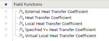
Figure 1: Available Heat Transfer Coefficient Field Functions in Simcenter STAR-CCM+
Heat Transfer Coefficient
Let’s start with the “obvious” choice: the field function simply called Heat Transfer Coefficient. This is a good option when the fluid temperature in the proximity of the surface is fairly uniform because you specify one reference temperature in the field function properties under Automation → Field Functions → Heat Transfer Coefficient (see Figure 2). Ideally, this reference should represent the bulk-fluid temperature around the surface from which you want to extract the HTC. With an appropriate reference temperature, the result is comparable to textbook values.
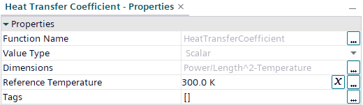
Figure 2: Setting the correct reference temperature for your flow conditions
However, if you have a complex temperature distribution in your domain, evaluating this function will be tedious, as you would have to adjust your reference temperature to each area before extracting the HTC.
For coupling to another solver, e.g. a 1D simulation tool, Simcenter STAR-CCM+ offers two HTC field functions that, to be applied correctly, need to be used in combination with their respective reference temperature function: The Specified Y+ HTC and the Local HTC. The HTC value alone may differ from a textbook coefficient, but the pair of HTC and its corresponding reference-temperature reproduces the heat flux across the boundary regardless.
Local Heat Transfer Coefficient
The Local HTC is calculated between the boundary and the first adjacent cell. Its value therefore depends strongly on the near-wall mesh and should not be compared directly with HTCs from a textbook. Its main advantage is that the corresponding Local HTC Reference Temperature explicitly accounts for effects such as radiation, which can make the pair useful when radiation is included in the simulation.
For multiphase continua there will be separate versions of the Local HTC, one for each phase. These can then be weighted by volume fraction and to be summed up to one value, to obtain a global HTC.
Specified Y+ Heat Transfer Coefficient
The Specified Y+ Heat Transfer Coefficient is a great option when you have varying temperature conditions in your domain, and you want a result that’s less mesh dependent compared to the Local Heat Transfer Coefficient. In the properties for this field function, you can pick a suitable y+ distance from the respective surfaces to evaluate the necessary parameters in. The default value is y+=100, hence it is sufficiently far away from the heat transfer surface not to be influenced by the near wall mesh resolution.
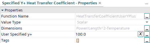
Figure 3: Specifying the dimensionless y+ value for the Specified Y+ HTC
The Specified Y+ HTC comes together with its own reference temperature, and both must be used combined in order to represent the correct heat flux from your simulation.
It is important to note that the reference temperature does not necessarily have to be your exact bulk temperature at the y+ distance you specify. Quite often, this will actually not be the case. The way Simcenter STAR-CCM+ calculates the Specified Y+ Heat Transfer Reference Temperature is as follows:
- Calculate the heat flux q” by solving the energy equation, which is a function of the friction velocity, wall temperature, your near-wall y+ and user-defined flow properties, such as density and heat capacity
- In the next step, the Specified Y+ HTC is calculated as a function of the non-dimensional temperature based on the user-specified y+ ( T^{+}=Pr_{t}y^{+}, if the first cell is in the viscous sublayer).
- In a last step, the Specified Y+ Heat Transfer Reference Temperature is calculated using:
T_{\textrm ref}=T_{\textrm surf}+\cfrac{q''}{h_{y^{+}}}
Hence, as you can see, the specified y+ location is only indirectly used for obtaining the reference temperature. This also means that very small changes to your flow field can have a large effect on the calculated reference temperature.
Let’s illustrate this by the following example: we have a domain with two regions with different ambient temperatures, and one temperature boundary in shape of a cylinder in each of them. As long as the regions are separated (upper figure), the flow fields are simple and there are no external influences on the cylinder boundary. The respective Specified Y+ Heat Transfer Reference Temperature is therefore equal to the ambient temperature. However, when connecting both regions with an interface (lower figure), the flow fields from both regions start to interact and the reference temperatures are affected, even if the flow and temperature fields in proximity to the specified y+ distance appear unchanged.
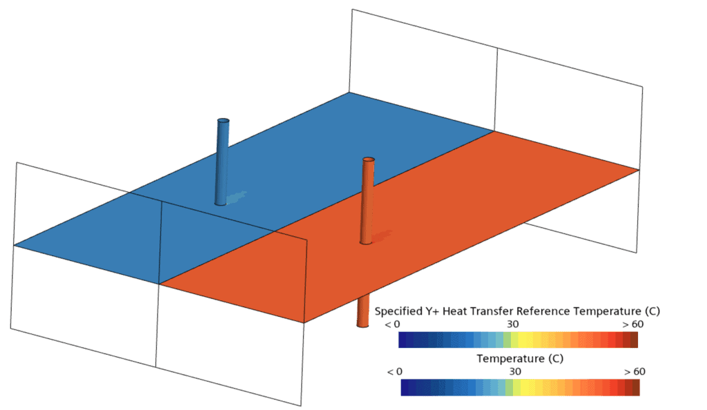
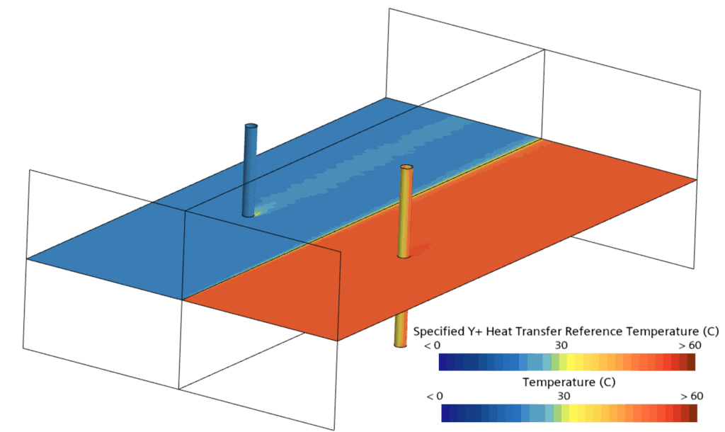
Figure 4: Example case with two warm cylinders in two regions with different ambient temperatures (upper: regions separated, lower: regions connected via an interface)
Another limitation is, that if you end up outside of your allowed temperature range (specified in the continuum), it will limit the reference temperature to Tmin or Tmax and the Specified Y+ HTC will be re-evaluated based on that new reference temperature to represent the correct heat flux.
If you want to know more about how the Specified Y+ Heat Transfer Reference Temperature is calculated in Simcenter STAR-CCM+, I recommend you to have a look at this Knowledge Base article.
As for the Local HTC, there will be separate Specified Y+ HTC field functions for each continuum in a multiphase flow simulation.
The remaining two functions are the Virtual Local HTC and the External HTC. They fulfill slightly different functions from the ones discussed so far. The Virtual Local HTC can be used to approximate the HTC, by skipping to solve the energy equation. The External HTC is user-specified as a boundary condition, so the field function allows double-checking on the correct implementation.
Virtual Local Heat Transfer Coefficient
This heat transfer coefficient can be useful when your main interest is to get an approximation of the heat transfer coefficient to your surface, but you’re not interested in the specific temperature distribution in your flow. Then you can skip solving the energy equation, but the pre-requisite for that is, that you have a well-defined reference temperature and that the heat flux is not expected to cause significant changes to the fluid temperature. Since the solver does not solve the energy equation, the specific heat, Cp, and the molecular and turbulent Prandtl numbers need to be correctly specified as reference values.
Like the Local HTC, the Virtual Local HTC evaluates heat transfer between the wall and the first near-wall cell centre, so it is mesh dependent. It is not recommended for laminar flow, and the first-cell y+ should remain between 30 and 100.
This function is not suitable for two-way coupling with other solvers.
External Heat Transfer Coefficient
This field function will only give you a result if you’re running your simulation with a “Convection” boundary condition on the surface of interest. Then you’ll specify your heat transfer coefficient as a constant/field function/table on your surface, e.g. as a result from a correlation study or similar. Hence, evaluating this field function is more of a sanity-check for your boundary conditions than a part of post-processing your results.
Summary
To summarize, picking the correct HTC field function and knowing how to use it has a big impact on how you can utilize your results, but hopefully this article has given you more clarity on the differences.
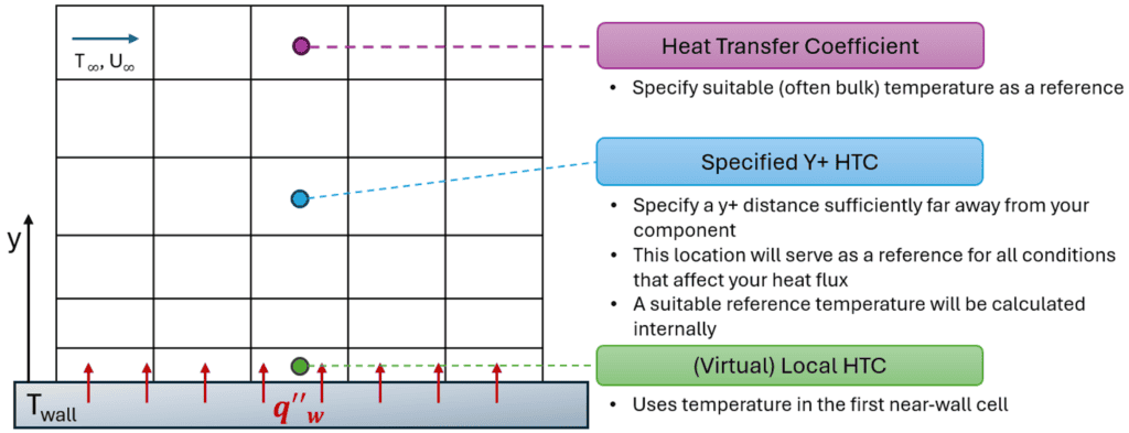
Figure 4: Overview of reference points for different HTC Field Functions
If you have any further questions, don’t hesitate to contact us at support@volupe.com !
Author
Randi Franzke
support@volupe.com