
To demonstrate coupled thermal and structural analysis in Simcenter Simlab, we use a cylindrical structure composed of four ring sections, one of which has a reduced thickness. The geometry is created in Simcenter Inspire. Thermal loading is applied as a surface convection condition, while the bottom face of Ring 1 is structurally constrained in a user-defined cylindrical coordinate system. A built-in Simcenter Simlab material is used. Figure 1 highlights the structure and shows it’s overall dimensions. The mesh and analysis setup use SI units.
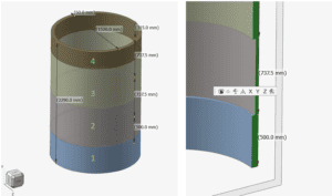
Figure 1: Model overview.
Use the default import settings. The geometry appears in the Assembly Browser, and any generated mesh is displayed with a .gda extension. You can define multiple mesh configurations, but only one mesh from a single assembly can be active at the same time, preventing meshes being mixed between assemblies. Additional model browsers are available at the bottom of the Assembly Browser.
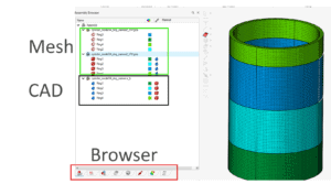
Figure 2: Works space overview, Imported CAD and meshed parts.
In this demo, we first merge the CAD parts into a single body and create a surface mesh, followed by a solid tetrahedral mesh. We then unmerge the mesh and verify node compatibility between the bodies using the Shared Faces command. The faces remain shared because the bodies were merged before meshing. To view the selected entities, enable the Selection Output List from View > Selection List.
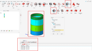
Figure 3: Merged CAD parts into one single body, note the selected parts in the selection list.
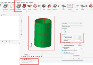
Figure 4: Surface mesh commands and Settings. The combined body is selected in the “Selection Output list”.
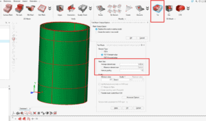
Figure 5: 3D Tet mesh of body, once meshing is performed, right click on body and select Unmerged.
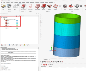
Figure 6: 3d meshed parts when unmerged are populated in the file tree.
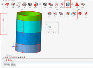
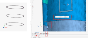
Figure 7: Check shared faces and mesh quality with section cut.
Next, define the solution. Switch to the Solutions Browser, open the Solutions tab, and select Coupled Solutions. By default, OptiStruct is selected as the solver and Structural and Electrical Analysis as the solution type. Select the meshed bodies by clicking them or using box selection, ensuring that all selected bodies belong to the same .gda mesh. Create two load cases by right-clicking Coupled under Solutions and selecting “Define Using Load Cases.” Create the second load case by copying the first or by right-clicking and adding another load case. Set the first load case to Type = “Steady State Heat Transfer” and the second to Type = “Linear Static.” This creates one thermal analysis and one structural analysis. For clarity, assign descriptive names such as “Thermal” and “Static.” To activate a load case, right-click it and select “Set Current.” The options available on the Solutions tab depend on which load case is current.
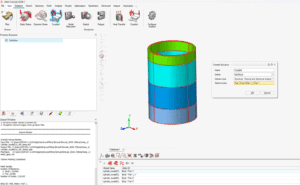
Figure 8: Solution tab and Coupled simulation (Solution set-up can be changed with the cogwheel Configure Solution).
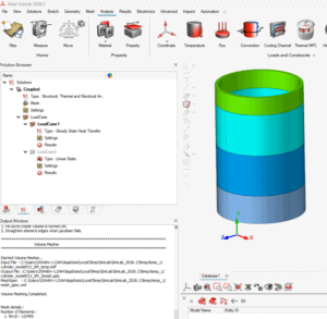
Figure 9: Subcase creation. Right click on load case setting will open micro dialog for creation of subcase output etc.
For the Thermal load case, ensure that it is current. Select the Convection icon and create two convection sets by selecting the required surfaces.
Next, make the Structural load case current and couple it to the Thermal load case. Right-click Settings, open Solution Settings, and select the Thermal load case for coupling. Constrain thermal expansion at the bottom face using a cylindrical coordinate system. To create the system, select System > Create, set Type to Cylindrical, and select a circular arc on the bottom face to define the centre. Assign all meshed bodies to the new coordinate system and set LCS Type to Analysis.
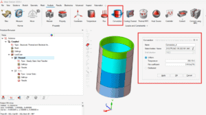
Figure 10: Convection set-up, two sets 5W/(m^2K) to 20C and 300W/(m^2K) to 400C. Cooling and heating respectively.
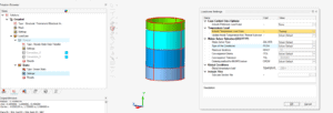
Figure 11: Coupling, link the Structural to the thermal load case.
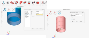
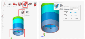
Figure 11: System and constraints definition.
Material assignment and property set-up are done in the next step. Built in material database is used and default “Steel” is used in this case!
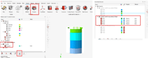
Figure 12: Material and property assignment. “Right Click” on bodies open up a micro dialog menu for easy assignment of material in the database.
After completing the setup, “Right-Click” on Results and select Update. The solver runs in the background, and the results become available when the analysis is complete.
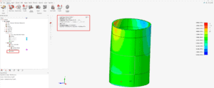
Figure 13: Postprocessing and evaluation of the results!
In the post processing micro dialog window, toggle between different loadcase and result type to explore the results in more detail.
Hopefully this has given you some insights how to work and model Structural cases in Simcenter Simlab!
As always, if you have questions about any other product in the Simcenter simulation portfolio, you can send us questions at support@volupe.com
Author

Johan Dahlberg
Contact: support@volupe.com
