Extracting wall adjacent field values in Simcenter STAR-CCM+

Johan BernanderSenior Application Specialist
In short
To evaluate a quantity at a set distance from a wall in Simcenter STAR-CCM+, enable the Wall Distance model, create an isosurface at that distance and map its values back to the wall. Our pipe example uses it for a heat transfer coefficient with the reference temperature 2.5 cm from the wall.
In this week’s blog post we will explain how to evaluate and extract field values at a specific distance from a wall boundary. As the basis for the methodology, we will use an example where we would like to evaluate a user-defined heat transfer coefficient, with a reference temperature extracted at a specific distance from the wall.
Heat Transfer Coefficient
The heat transfer coefficient, often denoted , is a proportionality constant that relates the heat flux across a boundary () to the temperature difference between the wall and a reference location (in the bulk flow). This relation is expressed by Newton’s law of cooling:
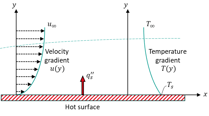
As understood from the relation above, the value of the reference location for the bulk temperature () will dictate the value of the heat transfer coefficient. In Simcenter STAR-CCM+ there are four different predefined options for the calculation of :
- Heat Transfer Coefficient
- Local Heat Transfer Coefficient
- Specified Y+ Heat Transfer Coefficient
- Virtual Heat Transfer Coefficient
Option 1 uses a user-defined single value reference temperature, option 2 uses the near wall cell temperature, and option 3 uses the cell temperature at a user-defined Y+ value (i.e. a specific location in, or outside, the boundary layer). Option 4 uses the wall treatment formulation to estimate the heat transfer coefficient based on empirical data and some user-specific input.
In this example, we want to define a fifth option, where the reference temperature is extracted at a user-specified distance from the wall boundary.
Extracting values off the wall
We’ll consider a simple circular pipe, 1 meter long and 20 cm in diameter, and run an air flow of 40°C and 1 m/s through the pipe. On the pipe wall there is an external heat transfer coefficient of 15 W/mK and an ambient temperature of 22°C.
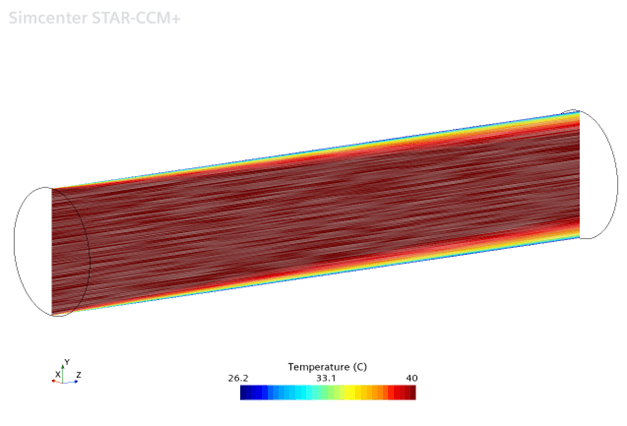
Now we want to evaluate the internal heat transfer coefficient based on a reference temperature 2.5 cm off the wall. To extract field values (in this case the temperature) at a specific distance from the wall, we will make use of the Wall Distance field function and an isosurface.
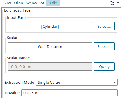
For the Wall Distance field function to be available, the Wall Distance model must be enabled in the Physics Continuum, as depicted below.

The isosurface can then be used to visualize or extract values at the specified wall distance. Below is a depiction of the temperature distribution on the isosurface and the cross-section of the pipe.
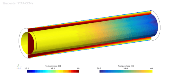
To extract each individual field value on the isosurface we make use of a table. We create an XYZ Internal Table and select the isosurface as the ingoing part. For this example the scalar field we want to extract is the temperature.
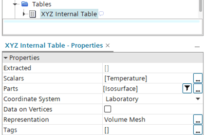
Once the table input is set, we right-click the table and select Extract.

Now we can see that the Extracted field is populated.
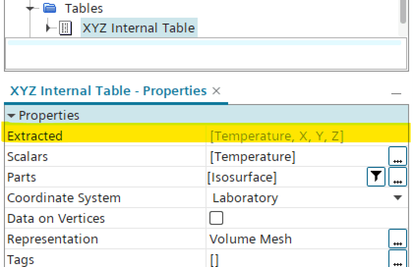
The table could now be exported for use in an external analysis, but in this case we want to use the extracted values in a field function for a user-defined heat transfer coefficient. To achieve this, we will make use of a Tabular Data Mapper.
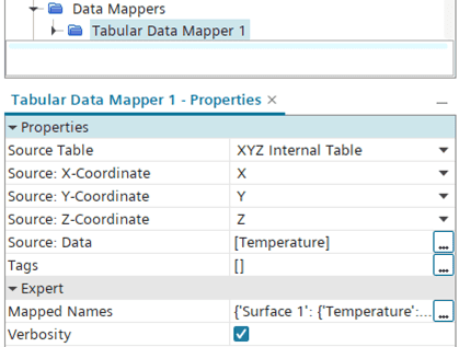
The target for our data mapper should be the pipe wall, meaning we will use a surface target. Then we specify the pipe (or “Cylinder”) wall as the Target Entity (see below).
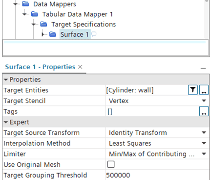
Now we can run the data mapper to generate the mapped temperature field function.
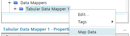
The mapped temperature field function is now ready to be used in the expression for our user-defined heat transfer coefficient. Here we decide to use an absolute value for the heat transfer coefficient, so that it always returns a positive value.

The resulting user-defined heat transfer coefficient distribution is depicted below.
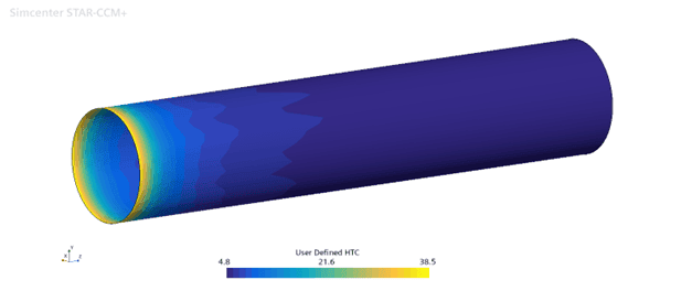
To check the validity of the calculated heat transfer coefficient, let’s compare it with the pre-defined Specified Y+ Heat Transfer Coefficient, which should be the most similar one in terms of definition. The picture below shows the difference between the two heat transfer coefficients.
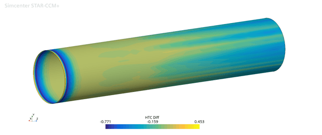
Seeing that the differences are comparably small, we can conclude that the user-defined heat transfer coefficient returns reasonable values.
As always, feel free to send any questions or comments to support@volupe.com.